2 Objects = Data + Function

One of the key concepts behind so-called object-oriented programming (OOP) is the notion of an object. An object is a new kind of value that can, as a first cut, be understood as a pairing together of two familiar concepts: data and function.

• An object is like a structure in that it has a fixed number of fields, thus an object (again, like a structure) can represent compound data. But unlike a structure, an object contains not just data, but functionality too;

• An object is like a (set of) function(s) in that it has behavior—it computes; it is not just inert data.

This suggests that objects are a natural fit for well-designed programs since good programs are organized around data definitions and functions that operate over such data. An object, in essence, packages these two things together into a single programming apparatus. This has two important consequences:

1. You already know how to design programs oriented around objects.

   Since objects are just the combination of two familiar concepts that you already use to design programs, you already know how to design programs around objects, even if you never heard the term “object” before. In short, the better you are at programming with functions, the better you will be at programming with objects.

2. Objects enable new kinds of abstraction and composition.

   Although the combination of data and function may seem simple, objects enable new forms of abstraction and composition. That is, objects open up new approaches to the construction of computations. By studying these new approaches, we can distill new design principles. Because we understand objects are just the combination of data and function, we can understand how all of these principles apply in the familiar context of programming with functions. In short, the better you are at programming with objects, the better you will be at programming with functions.

In this chapter, we will explore the basic concepts of objects by revisiting a familiar program, first organized around data and functions and then again organized around objects.

2.1 Functional rocket

In this section, let’s develop a simple program that animates the lift-off of a rocket.

The animation will be carried out by using the big-bang system of the 2htdp/universe library. For an animation, big-bang requires settling on a representation of world states and two functions: one that renders a world state as an image, and one that consumes a world state and produce the subsequent world state.

Generically speaking, to make an animation we must design a program of the form:

(big-bang <world0>           ; World

(on-tick <tick>)   ; World -> World

(to-draw <draw>))  ; World -> Scene

where World is a data definition for world states, <tick> is an expression whose value is a World -> World function that computes successive worlds and <draw> is an expression whose value is a World -> Scene function that renders a world state as an image.

For the purposes of a simple animation, the world state can consist of just the rocket:

;; A World is a Rocket.

The only relevant piece of information that we need to keep track of to represent a rocket lifting off is its height. That leads us to using a single number to represent rockets. Since rockets only go up in our simple model, we can use non-negative numbers. We’ll interpret a non-negative number as meaning the distance between the ground and the (base of the) rocket measured in astronomical units (AU):

;; A Rocket is a non-negative Number.

;; Interp: distance from the ground to base of rocket in AU.

This dictates that we need to develop two functions that consume Rockets:

;; next : Rocket -> Rocket

;; Compute next position of the rocket after one tick of time.

;; render : Rocket -> Scene

;; Render the rocket as a scene.

Let’s take them each in turn.

2.1.1 The next function

For next, in order to compute the next position of a rocket we need to settle on the amount of elapsed time a call to next embodies and how fast the rocket rises per unit of time. For both, we define constants:

(define CLOCK-SPEED  1/30) ; SEC/TICK

(define ROCKET-SPEED 1)    ; AU/SEC

The CLOCK-SPEED is the rate at which the clock ticks, given in seconds per tick, and ROCKET-SPEED is the rate at which the rocket lifts off, given in AU per second. We use these two constants to define a third, computed, constant that gives change in the rocket’s distance from the ground per clock tick:

(define DELTA (* CLOCK-SPEED ROCKET-SPEED)) ; AU/TICK

We can now give examples of how next should work. We are careful to write test-cases in terms of the defined constants so that if we revise them later our tests will still be correct:

(check-expect (next 10) (+ 10 DELTA))

Now that we have develop a purpose statement, contract, and example, we can write the code, which is made clear from the example:

;; next : Rocket -> Rocket

;; Compute next position of the rocket after one tick of time.

(check-expect (next 10) (+ 10 DELTA))

(define (next r)

(+ r DELTA))

2.1.2 The render function

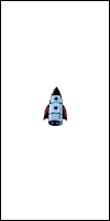
The purpose of render is visualize a rocket a scene. Remember that rockets are represented by the distance between the ground and their base, so a rocket at height 0 should sitting at the bottom of a scene. We want it to look something like:

> (render 0)

To do so we need to settle on the size of the sceen and the look of the rocket. Again, we define constants for this. We use the 2htdp/image library for constructing images.

(define ROCKET ) ; Use rocket key to insert the rocket here.

(define WIDTH 100)   ; PX

(define HEIGHT 200)  ; PX

(define MT-SCENE (empty-scene WIDTH HEIGHT))

You can copy and paste the rocket image from this program, or you can access the image as follows:

> (bitmap class/0/rocket.png)

Since we may want to draw rockets on scenes other than the MT-SCENE, let’s develop a helper function:

;; draw-on : Rocket Scene -> Scene

;; Draw rocket on to scene.

(define (draw-on r scn) ...)

allowing us to define render simpy as:

;; render : Rocket -> Scene

;; Render the rocket as a scene.

(define (render r)

(draw-on r MT-SCENE))

Recall that a rocket is represented by the distance from the ground to its base. On the other hand, the 2htdp/image library works in terms of pixels (PX) and graphics coordinates. We need draw-on to establish the mapping between AU. For simplicity, we assume 1 PX equals 1 AU. Using overlay/align/offset, the draw-on functions places the rocket on the scene on the center, bottom of the scene, offset vertically by the height of the rocket:

;; draw-on : Rocket Scene -> Scene

;; Draw rocket on to scene.

(define (draw-on r scn)

(overlay/align/offset "center" "bottom"

ROCKET

0 (add1 r)

scn))

2.1.3 Lift off

With these functions in place, let’s launch a rocket:

;; Lift off!

(big-bang 0

(tick-rate CLOCK-SPEED)

(on-tick next)

(to-draw render))

Our complete BSL program is:

(require 2htdp/image)

(require 2htdp/universe)

; A World is a Rocket.

; A Rocket is a non-negative Number.

; Interp: distance from the ground to base of rocket in AU.

(define CLOCK-SPEED  1/30) ; SEC/TICK

(define ROCKET-SPEED 1)    ; AU/SEC

(define DELTA (* CLOCK-SPEED ROCKET-SPEED)) ; AU/TICK

(define ROCKET ) ; Use rocket key to insert the rocket here.

(define WIDTH 100)   ; PX

(define HEIGHT 200)  ; PX

(define MT-SCENE (empty-scene WIDTH HEIGHT))

; next : Rocket -> Rocket

; Compute next position of the rocket after one tick of time.

(check-expect (next 10) (+ 10 DELTA))

(define (next r)

(+ r DELTA))

; render : Rocket -> Scene

; Render the rocket as a scene.

(define (render r)

(draw-on r MT-SCENE))

; draw-on : Rocket Scene -> Scene

; Draw rocket on to scene.

(check-expect (draw-on 0 (empty-scene 100 100))

(overlay/align/offset "center" "bottom"

ROCKET

0 1

(empty-scene 100 100)))

(define (draw-on r scn)

(overlay/align/offset "center" "bottom"

ROCKET

0 (add1 r)

scn))

; Lift off!

(big-bang 0

(tick-rate CLOCK-SPEED)

(on-tick next)

(to-draw render))

2.2 Object-oriented rocket

Now let’s redevelop this program only instead of using data and functions, we’ll use objects.

You’ll notice that there are two significant components to the rocket program. There is the data, which in this case is a number representing the distance the rocket has traveled, and the functions that operate over that class of data, in this case next and render.

This should be old-hat programming by now. But in this book, we are going to explore a new programming paradigm that is based on objects. As a first approximation, you can think of an object as the coupling together of the two significant components of our program (data and functions) into a single entity: an object.

Since we are learning a new programming language, you will no longer be using BSL and friends. Instead, select Language|Choose Language... in DrRacket, then select the “Use the language declared in the source” option and add the following to the top of your program:

#lang class/0

The constants of the rocket program remain the same, so our new program still includes a set of constant definitions:

(define CLOCK-SPEED  1/30) ; SEC/TICK

(define ROCKET-SPEED 1)    ; AU/SEC

(define DELTA (* CLOCK-SPEED ROCKET-SPEED)) ; AU/TICK

(define ROCKET ) ; Use rocket key to insert the rocket here.

(define WIDTH 100)   ; PX

(define HEIGHT 200)  ; PX

(define MT-SCENE (empty-scene WIDTH HEIGHT))

A set of objects is defined by a class, which determines the number and name of fields and the name and meaning of each behavior that every object is the set contains. By analogy, while an object is like a structure, a class definition is like a structure definition.

2.2.1 A class of rockets

The way to define a class is with define-class:

(define-class rocket%

(fields dist))

This declares a new class of values, namely rocket% objects. (By convention, we will use the % suffix for the name of classes.) For the moment, rocket% objects consist only of data: they have one field, the dist between the rocket and the ground.

This creates a rocket% representing a rocket with height 7.

In order to access the data, we can invoke the dist accessor method. Methods are like functions for objects and they are called by using the send form like so:

> (send (new rocket% 7) dist)

7

This suggests that we can now re-write the data definition for Rockets:

;; A Rocket is a (new rocket% NonNegativeNumber)

;; Interp: distance from the ground to base of rocket in AU.

2.2.2 The next and render methods

To add functionality to our class, we define methods using the define form. In this case, we want to add two methods next and render:

;; A Rocket is a (new rocket% NonNegativeNumber)

;; Interp: distance from the ground to base of rocket in AU.

(define-class rocket%

(fields dist)

;; next : ...

(define (next ...) ...)

;; render : ...

(define (render ...) ...))

We will return to the contracts and code, but now that we’ve seen how to define methods, let’s look at how to apply them in order to actually compute something. To call a defined method, we again use the send form, which takes an object, a method name, and any arguments to the method:

(send (new rocket% 7) next ...)

This will call the next method of the object created with (new rocket% 7). This is analogous to applying the next function to 7 in the Functional rocket section. The elided code (...) is where we would write additional inputs to the method, but it’s not clear what further inputs are needed, so now let’s turn to the contract and method headers for next and render.

When we designed the functional analogues of these methods, the functions took as input the rocket on which they operated, i.e. they had headers like:

;; next : Rocket -> Rocket

;; Compute next position of the rocket after one tick of time.

;; render : Rocket -> Scene

;; Render the rocket as a scene.

But in an object, the data and functions are packaged together. Consequently, the method does not need to take the world input; that data is already a part of the object and the values of the fields are accessible using accessors. In other words, methods have an implicit input that does not show up in their header—it is the object that has called the method. That value, since it is not available as an explicit parameter of the method, is made available through the this variable. We likewise revise the purpose statements to reflect the fact “the rocket” is the object calling the method, so we instead write “this rocket”, emphasizing that this refers to a rocket.

That leads us to the following method headers:

rocket%

;; next : -> Rocket

;; Compute next position of this rocket after one tick of time.

(define (next) ...)

;; render : -> Scene

;; Render this rocket as a scene.

(define (render) ...)

The rocket% box is our way of saying that this code should live in the rocket% class.

Since we now have contracts and have seen how to invoke methods, we can now formulate test cases:

rocket%

;; next : -> Rocket

;; Compute next position of this rocket after one tick of time.

(check-expect (send (new rocket% 10) next)

(new rocket% (+ 10 DELTA)))

(define (next) ...)

;; render : -> Scene

(check-expect (send (new rocket% 0) render)

(overlay/align/offset "center" "bottom"

ROCKET

0 1

MT-SCENE))

(define (render) ...)

Finally, we can write the code from our methods:

rocket%

(define (next)

(new rocket% (+ (send this dist) DELTA)))

(define (render)

(send this draw-on MT-SCENE))

Just as in the functional design, we choose to defer to a helper to draw a rocket on to the empty scene, which we develop as the following method:

rocket%

;; draw-on : Scene -> Scene

;; Draw this rocket on to scene.

(define (draw-on scn)

(overlay/align/offset "center" "bottom"

ROCKET

0 (add1 (send this dist))

scn))

At this point, we can construct rocket% objects and invoke methods.

2.2.3 A big-bang oriented to objects

It’s now fairly easy to construct a program using rocket% objects that is of the generic form of a big-bang animation:

(big-bang <world0>           ; World

(on-tick <tick>)   ; World -> World

(to-draw <draw>))  ; World -> Scene

We can again define a world as a rocket:

;; A World is a Rocket.

This creates the desired animation, but something should stick out about the above code. The big-bang system works by giving a piece of data (a number, a position, an image, an object, etc.), and a set of functions that operate on that kind of data. That sounds a lot like... an object! It’s almost as if the interface for big-bang were designed for, but had to fake, objects.

Now that we have objects proper, we can use a new big-bang system has an interface more suited to objects. To import this OO-style big-bang, add the following to the top of your program:

(require class/universe)

In the functional setting, we had to explicitly give a piece of data representing the state of the initial world and list which functions should be used for each event in the system. In other words, we had to give both data and functions to the big-bang system. In an object-oriented system, the data and functions are already packaged together, and thus the big-bang form takes a single argument: an object that both represents the initial world and implements the methods needed to handle system events such as to-draw and on-tick.

So to launch our rocket, we simply do the following:

(big-bang (new rocket% 0))

In order to handle events, we need to add the methods on-tick and to-draw to rocket%:

rocket%

;; on-tick : -> World

;; Tick this world

(define (on-tick) ...)

;; to-draw : -> Scene

;; Draw this world

(define (to-draw) ...)

These methods, for the moment, are synonymous with next and render, so their code is simple:

rocket%

(define (on-tick) (send this next))

(define (to-draw) (send this render))

Our complete program is:

#lang class/0

(require 2htdp/image)

(require class/universe)

; A World is a Rocket.

; A Rocket is a (new rocket% NonNegativeNumber).

; Interp: distance from the ground to base of rocket in AU.

(define CLOCK-SPEED  1/30) ; SEC/TICK

(define ROCKET-SPEED 1)    ; AU/SEC

(define DELTA (* CLOCK-SPEED ROCKET-SPEED)) ; AU/TICK

(define ROCKET ) ; Use rocket key to insert the rocket here.

(define WIDTH 100)   ; PX

(define HEIGHT 200)  ; PX

(define MT-SCENE (empty-scene WIDTH HEIGHT))

(define-class rocket%

(fields dist)

; next : -> Rocket

; Compute next position of this rocket after one tick of time.

(check-expect (send (new rocket% 10) next)

(new rocket% (+ 10 DELTA)))

(define (next)

(new rocket% (+ (send this dist) DELTA)))

; render : -> Scene

; Render this rocket as a scene.

(check-expect (send (new rocket% 0) render)

(overlay/align/offset "center" "bottom"

ROCKET

0 1

MT-SCENE))

(define (render)

(send this draw-on MT-SCENE))

; draw-on : Scene -> Scene

; Draw this rocket on to scene.

(define (draw-on scn)

(overlay/align/offset "center" "bottom"

ROCKET

0 (add1 (send this dist))

scn))

; on-tick : -> World

; Tick this world

(define (on-tick) (send this next))

; to-draw : -> Scene

; Draw this world

(define (to-draw) (send this render)))

; Lift off!

(big-bang (new rocket% 0))

You’ve now seen the basics of how to write programs with objects.

2.3 A Brief History of Objects

Objects are an old programming concept that first appeared in the late 1950s and early 1960s just across the Charles river at MIT in the AI group that was developing Lisp. Simula 67, a language developed in Norway as a successor to Simula I, introduced the notion of classes. In the 1970s, Smalltalk was developed at Xerox PARC by Alan Kay and others. Smalltalk and Lisp and their descendants have influenced each other ever since. Object-oriented programming became one of the predominant programming styles in the 1990s. This coincided with the rise of graphical user interfaces (GUIs), which objects model well. The use of object and classes to organize interactive, graphical programs continues today with libraries such as the Cocoa framework for Mac OS X.

2.4 Exercises

2.4.1 Complex, with class

(part "Complex_with_class_solution")

For this exercise, you will develop a class-based representation of class-based representation ofcomplex numbers, which are used in several fields, including: engineering, electromagnetism, quantum physics, applied mathematics, and chaos theory.

A complex number is a number consisting of a real part and an imaginary part. It can be written in the mathematical notation a+bi, where a and b are real numbers, and i is the standard imaginary unit with the property i2 = −1.

Supposing your language was impoverished and didn’t support complex numbers, you should be able to build them yourself since complex numbers are easily represented as a pair of real numbers—the real and imaginary parts.

Design a structure-based data representation for Complex values. Design the functions =?, plus, minus, times, div, sq, mag, and sqroot. Finally, design a utility function to-number which can convert Complex values into the appropriate Racket complex number. Only the code and tests for to-number should use Racket’s complex (non-real) numbers and arithmetic since the point is to build these things for yourself. However, you can use Racket to double-check your understanding of complex arithmetic.

For mathematical definitions of complex number operations, see the Wikipedia entries on complex numbers and the square root of a complex number.

> (define c-1  (make-cpx -1 0))

> (define c0+0 (make-cpx 0 0))

> (define c2+3 (make-cpx 2 3))

> (define c4+5 (make-cpx 4 5))

> (=? c0+0 c0+0)

#t

> (=? c0+0 c2+3)

#f

> (=? (plus c2+3 c4+5)       (make-cpx 6 8))

#t

Develop a class-based data representation for Complex values. Add accessor methods for extracting the real and imag parts. Develop the methods =?, plus, minus, times, div, sq, mag, sqroot and to-number.

1.1 Circles

For this exercise, you will develop a structure-based representation of circles and functions that operate on circles, and then develop a class-based representation of circles.

A circle has a radius and color. They also have a position, which is given by the coordinates of the center of the circle (using the graphics coordinates system).

1. The circ structure and functions.

   Design a structure-based data representation for Circle values.

   Design the functions =?, area, move-to, move-by, stretch, draw-on, to-image, within?, overlap?, and change-color.

   Here are a few examples to give you some ideas of how the functions should work (note you don’t necessarily need to use the same structure design as used here).

   First, let’s define a few circles we can use:

   > (define c1 (make-circ 25 "red" 100 70))

   > (define c2 (make-circ 50 "blue" 90 30))

   > (define c3 (make-circ 10 "green" 50 80))

   A (make-circ R C X Y) is interpreted as a circle of radius R, color C, and centered at position (X,Y) in graphics-coordinates.

   The to-image function turns a circle into an image:

   > (to-image c1)

   > (to-image c2)

   > (to-image c3)

   While the draw-on function draws a circle onto a given scene:

   > (draw-on c1 (empty-scene 200 200))

   > (draw-on c2 (empty-scene 200 200))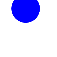

   > (draw-on c3 (empty-scene 200 200))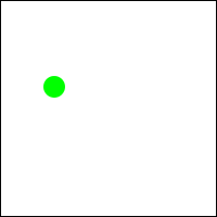

   > (draw-on c1 (draw-on c2 (draw-on c3 (empty-scene 200 200))))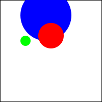

   The area function computes the area of a circle:

   > (area c1)

   1963.4954084936207

   > (area c2)

   7853.981633974483

   > (area c3)

   314.1592653589793

   The move-to function moves a circle to be centered at the given coordinates:

   > (draw-on (move-to c1 100 100) (empty-scene 200 200))

   While move-by moves a circle by the given change in coordinates:

   > (draw-on (move-by c1 -30 20) (empty-scene 200 200))

   The within? function tells us whether a given position is located within the circle; this includes any points on the edge of the circle:

   > (within? c1 (make-posn 0 0))

   #f

   > (within? c1 (make-posn 110 80))

   #t

   The change-color function produces a circle of the given color:

   > (to-image (change-color c1 "purple"))

   The =? function compares two circle for equality; two rectangles are equal if they have the same radius and center point—we ignore color for the purpose of equality:

   > (=? c1 c2)

   #f

   > (=? c1 c1)

   #t

   > (=? c1 (change-color c1 "purple"))

   #t

   The stretch function scales a circle by a given factor:

   > (draw-on (stretch c1 3/2) (empty-scene 200 200))

   The overlap? function determines if two circles overlap at all:

   > (overlap? c1 c2)

   #t

   > (overlap? c2 c1)

   #t

   > (overlap? c1 c3)

   #f

2. The circ% class.

   Develop a class-based data representation for Circle values. Develop the methods corresponding to all the functions above.

   The methods should work similar to their functional counterparts:

   > (define c1 (new circ%  25 "red" 100 70))

   > (define c2 (new circ% 50 "blue" 90 30))

   > (send c1 area)

   1963.4954084936207

   > (send c1 draw-on (empty-scene 200 200))