Due Wednesday Feb 19 Due Monday Feb 24, 11pm
Worth: 14% of your final grade
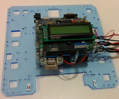
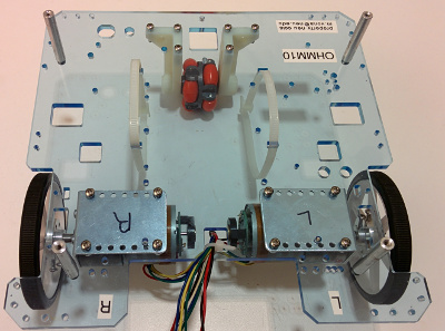
In the first part of this lab you’ll assemble the proximity sensors on your robot: two forward-facing bump switches and two side-facing infrared distance sensors.
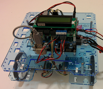
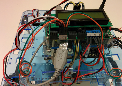
You will also add the PandaBoard processor which runs Ubuntu 12.04. The low-level processor (LLP, the Orangutan SVP board, or just the “org”) will now communicate with the pandaboard (the HLP, or just the “panda”) over a short USB cable on the robot. The pandaboard will take the place of the laptop or other external computer you have been using to communicate with the org. You will now connect to the HLP either via a USB-to-serial cable or over the network (wifi or Ethernet).
In the second part of the lab you’ll write code for the HLP to implement a form of local navigation based on the Bug2 algorithm.
In the third part of the lab you’ll write code for the HLP to implement a global navigation algorithm given a map. Your solutions for each part can make use of a library of supporting Java code
- HLP (PandaBoard)
- Get a PandaBoard, short USB A to mini-B cable, USB-to-serial adapter, and USB-wifi dongle. Make sure to take the components numbered for your lab group. Also get the PandaBoard cooling fan, power cable, and an extra USB socket with 2 4-40x3/8" screws.
- Disconnect and remove any USB cable currently connected to the LLP on your robot. Disconnect the battery and any AC supply to the robot, and remove the battery from the robot (you can leave the battery zipties on the robot).
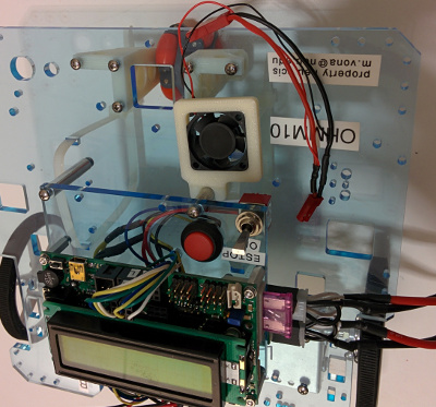
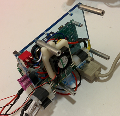
- Carefully attach the cooling fan to the right rear standoff on the electronics stack. You may need to push fairly hard. Make sure the fan is oriented correctly—its label should face down.
- Unhook the motor and encoder wires from the Orangutan board. Do not unhook the thicker power wires.
- Carefully remove the four screws holding the electronics stack from underneath the bottom plate. Keep track of them, you’ll need them again in a moment.
- Attach the extra USB socket to the front left of the electronics stack.
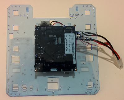
- The PandaBoard comes in a static protection bag. Trying to hold the board only by the edges, remove it carefully from the bag. Return the bag to the course staff so that we can reuse them.
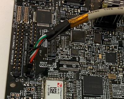
- Attach the extra USB socket to the pandaboard expansion connector near where it is labelled “J6” on the PandaBoard. The red wire should be to the right
 .
.
- Thread the fan power wires under the electronics stack mezzanine board (the blue plastic board under the Orangutan) and out towards the right side of the robot. Gently swing the fan around so that it is under the mezzanine board. This will put it over the PandaBoard CPU in the final assembly. Examine how the red fan power connector attaches underneath the Orangutan board. You don’t need to plug it in now—it makes a whining sound. It may be useful later in the course when the Orangutan board is doing image processing. Please use the pliers to unplug this connector instead of pulling on the wires.
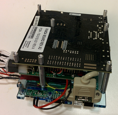
- Locate the pattern of three extra mounting holes on the PandaBoard, and notice that the front left (robot right) hole has three extra 4-40x3/8" standoffs on it. Use those to carefully attach the pandaboard to the bottom of the electronics stack. Be careful not to scratch the PandaBoard while you do this. Also watch out that the fan does not knock into any components on the PandaBoard, you may need to push it up a little.
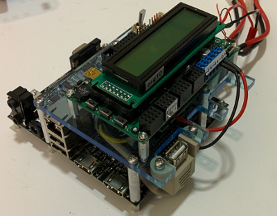
- Use the four screws you had removed from the electronics stack to mount the pandaboard to the top plate. Be careful to orient the top plate correctly and to use the correct holes.
- Attach the short USB cable from the LLP to the extra USB connector.
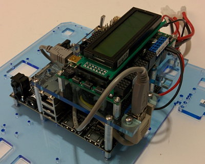
- Attach the HLP power cable from the rear socket on the Orangutan board to the PandaBoard.
- Top Plate
- Get 4 4-40x1.5" metal standoffs and 8 4-40x3/8" screws.
- Assemble the standoffs to the bottom plate using 4 of the screws in the indicated holes.
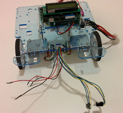
- Attach the top plate using the remaining 4 screws. Feed the motor and encoder wires up through the square hole in the front of the top plate and reconnect them to the Orangutan board as in LAB 1. Make sure the left motor red/black wires are connected to the left motor driver outputs, and similar for the right motor. Crossing the left and right motor connections can cause damage to the Orangutan board.
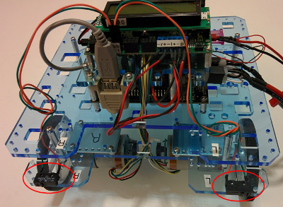
- Bump Switches
- Get two bump switches and four 4-40x3/8" screws.
- Assemble the bump switches on the front left and right of the bottom plate.
- Route the wires up through the square holes in the front corners of the top plate. Insert the left bump switch connector into the A0 port on the LLP marked
 and the right bump switch connector into the A1 port marked
 . The polarity of these connectors doesn’t matter (i.e. it doesn’t matter which color wire is forward). However, for the IR sensors which have similar connectors, polarity will matter.
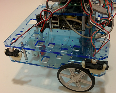
- IR Sensors
- Get two IR sensor assemblies and four 2-56x7/16" screws.
- Assemble the IR sensors on the right front and rear of the bottom plate. Make sure to orient them with the sensors facing out.
- Route the wires up through the square holes in the front and rear left side corners of the top plate. Insert the front IR connector into the A2 port on the LLP marked
 and the rear IR connector into the A3 port marked
 . Here the polarity (the way you insert the 3 pin connector, there are two possibilities) does matter. The black wire should be closest to the front of the robot, the red wire in the middle, and the white wire in the back (this also puts the white wire closest to the LCD).
- SD Card and Battery
- Have the course staff check your connections. You will then receive an SD card holding the HLP’s filesystem.
- Reattach the battery to the robot.
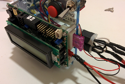
The HLP should boot once it receives power and as long as the SD card, which acts like its disk drive, is inserted (please don’t ever remove it after it is first installed). You should see the two LEDs near the SD card flash; you will likely become familiar with the pattern.
Important: once the HLP has booted, it is important to cleanly shut it down. This ensures that the filesystem on the SD card is left in a clean state. The HLP gets power from the LLP, so anytime you shut down the LLP, the HLP will also lose power. (It is ok to reset the LLP, as this does not affect its power supply circuitry.) The correct way to shut down the HLP is to log in to it (see below on different options for that) and run the command
> sudo shutdown -h now
Wait for the LED indicator lights near the SD card to stop flashing. It is then safe to remove power. Or, if you want to reboot the HLP:
> sudo shutdown -r now
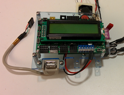
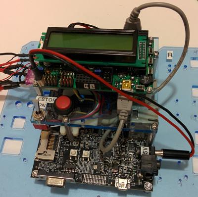
We have configured Ubuntu 12.04 on the HLP in a similar configuration to the ohmmkeys (VMWare is not involved here, of course). In place of the long black USB cables you were using to connect from the ohmmkey VM (or your own machine) to the LLP, we have now installed a short grey USB cable that connects the LLP to the HLP. The LLP communication port still appears at /dev/ttyACM1 on the HLP.
It is possible to use the HLP with a standard USB keyboard, mouse, and HDMI or DVI-D (but not VGA) display. The first two can be plugged in to any free USB port on the HLP. The display must connect to the HDMI connector labeled HDMI-1080p (the one further from the front of the robot). You may use either HDMI to HDMI or HDMI to DVI-D cables (VGA is unfortunately not supported without extra conversion electronics), but beware that the HLP may have configuration issues with some monitors. When using a monitor, it is best to have it connected at boot. We have had good results with 1280x1024 LCD panels.
It is more common to use the HLP in a “headless” mode where we only connect to it over the network—it has both wifi and Ethernet connections—and/or via a serial terminal connected to the RS-232 serial port on the DB-9 connector at the rear of the HLP. Because most computers no longer have true RS232 serial hardware, we provide you with a USB to serial adapter cable. You interact with this again using a terminal program such as kermit or minicom, but be aware that the port name will not be ACM1 here as it was for communicating directly with the LLP. The port name will depend on your system, typically on Linux it will be /dev/ttyUSB0, and on OSX it will be /dev/tty.usbserial. The adapter we provide is based on the Prolific PL2303 chipset, which should work without extra drivers at least on modern Linux installations. For other OS you may need to manually install drivers.
You may be familiar with GUI tools, including NetworkManager in Ubuntu, to identify and connect to wireless networks. Normally you interact with NM graphically via an icon in the task tray, but it is also possible to manipulate it from the command line. It runs as a daemon (background service) even when headless.
Please read carefully the information here about connecting the HLP to wifi networks from the command line. Also follow the instructions given in lab on the particulars of using the wifi on our networks.
The USB-wifi dongle we have provided you is not intended to be attached to the HLP, which has its own onboard wifi hardware. Instead, it is to be used with your ohmmkey or other virtual (or physical) machines used for code development and debugging. The dongle enables your development machine (or VM) to connect to the same wifi router as the HLP so that it can see the HLP’s local IP address when the router is using NAT (network address translation) to form a private subnet. It is probably not needed if your development machine is a laptop (whether or not you are using a VM)—in that case just connect your laptop directly to the same network to which your robot is connected.
There are three main ways to “log in” to the LLP:
Determine the IP address and the wifi network to which the HLP is connected. As described here, you can generally do this by pushing the user pushbutton on the HLP for about 1 second. The network name and the IP address will then appear on the LCD in a few sconds. Then, from another computer on the same network (or which can at least “see” the IP address of the HLP), ssh to it:
> ssh USER@IP
Here USER is your username on the HLP and IP is the IP address of the HLP. You can omit the USER@ part if your username on the HLP is the same as your username on the machine from which you are sshing. And you can also try
> ssh USER@ohmmN # N is your group number, USER@ is optional
or
> ssh USER@ohmmN.local # N is your group number, USER@ is optional
which in some cases, depending on configuration of the wifi network, allow you to use the name of your LLP instead of its IP address.
Connect the USB-serial adapter and then run
> minicom usb0
on your development machine, assuming you are running Linux and you have installed the provided minirc.usb0 in /etc/minicom or as ~/.minirc.usb0.
Attach a keyboard, mouse, and monitor, and log in graphically. You may need to reboot the HLP with the extra hardware connected.
Log in to the HLP with the “ohmm” account and add users for each of your group members just as you did for your ohmmkey in Lab 0 (though here the command line is probably going to be the way to go).
First, make SVN checkouts in your account on the HLP as described in lab 0.
Also, update any svn checkouts you already have on your ohmmkey or your personal development machines with a command like this:
> cd ~/robotics; svn up ohmm-sw; svn up ohmm-sw-site; svn up g0
Then follow similar instructions to copy the lab 2 framework as for lab 0, but change l0 to l2 in the instructions (do not delete your old l0-1 directories).
Please do not edit the provided files, in part because we will likely be posting updates to them. Any edits you make in them will be overwritten if/when you re-copy them to get our updates.
We have now included our solution for the LLP drive module in robotics/ohmm-sw-site/llp/monitor/drive.c and robotics/ohmm-sw-site/llp/monitor/ohmm/drive.h. To use this code, rebuild the monitor and flash it to your LLP. With the LLP connected and powered up (this should be the default if you are running these commands on the HLP), run these commands:
> cd ~/robotics/ohmm-sw/llp/monitor
> make clean; make; make program
If you would like to continue using your lab 1 solution code for the drive module instead of our solution, instead run these commands:
> cd ~/robotics/ohmm-sw/llp/monitor
> make clean; make lib IGNORE_DRIVE_MODULE=1
> cd ~/robotics/gN/l1; make; make program
However, you should be aware that the Java library we provide to talk to the monitor assumes that the drive module commands are implemented exactly as specified. Also, our solution for the drive module includes many additional commands beyond those you were required to write in lab 1. Solutions to future labs may assume that all the drive module commands from our solution are available.
We have also now included a Java library to run on the HLP and communicate with the monitor program running on the LLP. This will let you write Java code for the HLP which, for example, can make a function call like ohmm.motSetVelCmd(0.5f, 0.5f) instead of manually typing msv 0.5 0.5 into minicom. It also provides an optional scheme layer where you can make the scheme function call (msv 0.5f 0.5f) to achieve the same result. Almost all of the monitor commands have corresponding Java and scheme function calls.
You first need to build the jar file for this Java library like this:
> cd ~/robotics/ohmm-sw/hlp/ohmm
> make clean; make; make project-javadoc; make jar
The will also generate documentation for the OHMM Java library in robotics/ohmm-sw/hlp/ohmm/javadoc-OHMM (the top level file is index.html); or you can view it online here.
Next you can compile the example code we provided to get you started with the lab:
> cd ~/robotics/gN/l2
> make
To run the example code, we recommend using the run-class script we provide:
> cd ~/robotics/gN/l2
> ./run-class OHMMShellDemo -r /dev/ttyACM1
run-class is a shell script that uses the makefile to help build a Java command line, including classpath and other flags. (It assumes that there is a suitable makefile in the current directory.) The first argument, here OHMMShellDemo, is the Java class containing the main() function, with or without a package prefix (here we could have also used l2.OHMMShellDemo); when the package is omitted it is inferred from the project directory structure. The remaining arguments, here -r /dev/ttyACM1, are passed as command line arguments to main().
The jarfile generated in ~/robotics/ohmm-sw/hlp/ohmm will have a name like OHMM-RNNN_YYYY-MM-DD.jar where NNN is the SVN revision number of the OHMM library you are using and YYYY-MM-DD is the current date. A symbolic link will also be made OHMM-newest.jar -> OHMM-RNNN_YYYY-MM-DD.jar. The jarfile is very inclusive, it packages up
- all the OHMM compiled java class files
- all the OHMM sourcecode
- all the OHMM javadoc
- all the contents of all the pure-Java dependency jars for the OHMM library, which can include jscheme, RXTX, and javacv (see
EXT_JARS in makefile.project for the current full list)
This means that if you want to use your own machine for Java development, all you should need to do is transfer the OHMM jar to that machine and include it in the classpath when you run the java compiler. You can even unpack the jar so you can read the sourcecode and browse the javadoc:
# assuming you have the OHMM jar in the current dir as OHMM-newest.jar
> mkdir OHMM-jar; cd OHMM-jar; jar xvf ../OHMM-newest.jar
# now subdir ohmm contains the OHMM java sourcecode
# and subdir javadoc-OHMM contains the OHMM javadoc
If you actually want to run your code on your own machine and test it (e.g. with the LLP connected using the long black USB cable), you will also need to manually install the native libraries (.so on linux, .dylib on OS X, .dll on Windows) that are required by any of the dependencies. In particular, RXTX requires a native library for serial port communication, and javacv (which is not actually needed for this lab) would need access to the native OpenCV libraries. Where (and how) these should be installed is system dependent.
The demo program uses JScheme to implement a scheme read-eval-print-loop (REPL) command line. You can launch it like this:
> cd ~/robotics/gN/l2
> ./run-class OHMMShellDemo -r /dev/ttyACM1
or like this:
> cd ~/robotics/ohmm-sw/hlp
> ./run-class OHMMShell -r /dev/ttyACM1
or like this:
> java -cp path/to/OHMM-newest.jar ohmm.OHMMShell -r /dev/ttyACM1
First try a command like
> (e 14b)
$1 = 14B
which just asks the LLP monitor to echo back the given byte value 14b. Or run
> (df 1000.0f)
to add a 1000mm forward drive command to the queue and start it (the robot will move!). The b and f suffixes force scheme to interpret numeric literals as byte and float datatypes; they are necessary so that JScheme can correctly match the scheme call to a Java function. If the suffixes were omitted, the literals would have been interpreted as int and double (due to the .0), respectively, which will not be automatically converted to the narrower types byte and float.
Examine all the provided *.scm and *.java sourcecode in robotics/gN/l2, robotics/ohmm-sw/hlp/ohmm, and robotics/ohmm-sw-site/hlp/ohmm so you understand what is available and how to use it.
You can use the demo program as a template for your own code. For example, you could copy OHMMShellDemo.java to L2.java like this:
> cd ~/robotics/gN/l2
> cp OHMMShellDemo.java L2.java
> svn add L2.java
Then open L2.java in your editor and follow the instructions in it to customize it. Finally, to compile and run:
> cd ~/robotics/gN/l2
> make
> run-class L2 -r /dev/ttyACM1 # or whatever command line arguments you need
Bring up an OHMMShell and run the following commands to configure the bump switches as digital sensors and the IRs as analog sensors (you may omit the comments):
> (scd io-a0 #t #f) ; sensor config digital - left bump switch on IO_A0
> (scd io-a1 #t #f) ; sensor config digital - right bump switch on IO_A1
> (scair ch-2 1) ; sensor config analog IR - front IR on A2
> (scair ch-3 1) ; sensor config analog IR - rear IR on A3
scd stands for “sensor config digital” and scair stands for “sensor config analog ir”; they correspond to monitor comands in the sense module. io-a0, ch-2, etc. are convenience scheme constants which identify particular input/output ports and analog-to-digital conversion channels on the LLP.
It is always essential to configure the sensor inputs like this before you use them. If you are writing Java code, you could write ohmm.senseConfigDigital(DigitalPin.IO_A0, true, false) instead of (scd io-a0 #t #f) and ohmm.senseConfigAnalogIR(AnalogChannel.CH_2, 1) instead of (scair ch-2 1).
Try out the bump switches:
> (srd io-a0) (srd io-a1) # sensor read digital
They should read #t when triggered and #f otherwise. Make sure that the left sensor corresponds to the first reading and the right sensor to the second.
Try out the IRs. Set up a reasonable object at a known distance between 8 and 80cm, then run
> (sra ch-2) (sra ch-3) # sensor read analog
They should out the distance in millimeters, plus or minus a few due to noise. Make sure that the front sensor corresponds to the first reading and the rear sensor to the second.
Now you will implement a simplified version of the Bug2 local navigation algorithm covered in L5. The simplifying assumptions are:
- there is at most one obstacle between the start and the goal
- the first obstacle surface encountered, if any, will be roughly perpendicular to the M-line
- obstacles are always rectangular, with a minimum side width at least 1.5 times the robot length
- the robot initial pose is
 in world frame
- the goal position world frame
 coordinate is no less than -0.5m and no more than +5m, and the
 coordinate of the goal position is 0
We strongly recommend you write all code for this lab in Java that runs on the HLP. If you prefer to use other languages, we will allow that, but you will need to write your own equivalent of the Java interface code we provide. There should be no need to write more AVR C code for the LLP for this lab.
Develop a graphical debugging system that shows a birds eye view of the robot operating in a workspace with global frame coordinates at at least covering
 and
and
 . This display must bring up a graphics window that shows the axes of world frame and the current robot pose updated at a rate of at least 1Hz. Arrange the graphics so that world frame
points to the right, world frame
points up, and
. This display must bring up a graphics window that shows the axes of world frame and the current robot pose updated at a rate of at least 1Hz. Arrange the graphics so that world frame
points to the right, world frame
points up, and
 is vertically centered in the window (and remember, your graphics must always show at least the minimum world area stated above).
Make sure that this can work over the network, somehow, even when the HLP is headless. We have provided a simple HTTP-based ImageServer and some example code that uses it in robotics/g0/l2/ImageServerDemo.java. You could extend this code to draw the required graphics which will be sent to a remote client using a standard web browser.
Another option would be to use remote X Window display. Though this can use significant network bandwidth, it requires no special code. Just open a regular window and draw your graphics.
You could also design your own client/server protocol. If you do run a server, whether it speaks the HTTP protocol or some protocol you design, be aware that there is a firewall running on the HLP. You can get info on it here, including how to disable it or poke a hole in it so that your server can take incoming connections. By default the port 8080 should be available for your use.
Remember that the network can be unreliable. Your navigation code (for all parts of the assignment) should continue to work even if the graphical display fails because of network issues (and/or you can have an option to run your code with no graphical display, just text debugging).
Another consideration you should make when designing your debug graphics system, if you are using the provided Java OHMM library, is that there can be only one instance of the OHMM object. See the discussion titled “Thread Safety” in the javadoc.
Write a program for the HLP that implements the Bug2 algorithm subject to the above simplifications, and that uses your graphical debugging system to show its progress. The goal location should not be hardcoded, rather, read the goal
coordinate from the first command line argument in floating point meters.
If your Java class to solve this part is called Bug2, you should be able to invoke it like this
> ./run-class Bug2 4.3
for a goal at
 . You will likely find this more manageable if you break the task into the following parts:
- Drive forward slowly until at least one bumper switch triggers, or until the goal is reached.
- If an obstacle is encountered, “line up” to it with small motions until both bumpers are triggered (remember you first need to call
ohmm.senseConfigDigital() on the appropriate pins, see the discussion above in Sensor Testing).
- Back up a fixed amount (e.g. 25cm) and turn left
 .
.
- Start reading the IRs (remember you first need to call
ohmm.senseConfigAnalogIR() on the appropriate channels (notice the final two characters in that API are I and R)). Plot their data points in your debug system. Devise a way to estimate the obstacle wall pose from the data points (we suggest you use the line fitting approach covered in L6).
- Start driving forward slowly. You may need to implement a controller (e.g. PD) that tries to maintain the distance to the wall and the parallelism of the robot with the wall.
- Monitor the IR readings to detect the obstacle corner.
- Once the corner is detected, execute a fixed sequence of motions that turn the robot
 (i.e. to the right) so that it should end up at roughly the same distance from the left obstacle wall.
- Continue as above to follow the obstacle boundary until the leave point is reached.
- Turn and drive to the goal.
Whether or not you choose to solve the problem as we suggested above, it is a requirement that your debug code show (at least)
- the current robot pose
- the world frame axes
- the goal location
- the cumulative IR data points; i.e. all data points collected so far must be plotted.
It is also a requirement that your program somehow report the following events:
- Obstacle hit point encountered.
- Obstacle corner encountered.
- Obstacle leave point encountered.
- Goal reached.
Now you will implement a global navigation algorithm of some type; the visibility graph and free space graph algorithms presented in L7 are reasonable options. You may make the following simplifying assumptions:
- obstacles are always rectangular
- the robot initial pose is
in world frame
- the robot is always operating inside an “arena” with a rectangular boundary
- the robot outline, for planning purposes, is an axis aligned (even though the robot itself may rotate) square centered at the robot reference point (origin of robot frame, i.e. the midpoint between the wheel contact points) with side length
 , where
 is the radius of the smallest circle, also centered at the robot reference point, that encloses the actual robot outline, and
 is a positive value up to 10cm
Procedure:
Write a program for the HLP that implements your global navigation algorithm by reading in a text map file in the format
xgoal ygoal
xmin0 xmax0 ymin0 ymax0
xmin1 xmax1 ymin1 ymax1
...
xminN xmaxN yminN ymaxN
where each token is a floating point number in ASCII decimal format (e.g. as accepted by Float.parseFloat() in Java). The first line gives the goal location in meters in world frame. Each subsequent line defines an axis-aligned rectangle in world frame meters (the rectangle sides are always parallel or perpendicular to the coordinate frame axes, never tilted). The first is the arena boundary, and the rest are obstacles. There may be any number of obstacles, including zero. The obstacles may intersect each other and the arena boundary.
Make sure your map file parser can handle arbitrary whitespace (space and tab characters) between values, extra whitespace at the beginning or end of a line, blank lines, values that include leading + and -, and values with and without decimal points. And remember the values are in meters.
If your Java class to solve this part is called GlobalNav and you have a map in the above format stored in a file called themap, you should be able to invoke it either like this
> ./run-class GlobalNav themap
if you accept the name of the map file on the command line; or like this, if you read the map from the standard input stream
> ./run-class GlobalNav < themap
We will leave most details up to you. However, it is required that you have similar graphical debug code for this part as for local navigation, and that here it must show (at least)
- the current robot pose
- the world frame axes
- the arena boundary (and since the arena boundary is read from the map file, this means that you must somehow be able to resize or rescale your graphics at runtime to show the whole arena)
- all obstacle boundaries
- the goal location.
It is also a requirement that your program somehow indicate when the goal has been reached.
You will be asked to demonstrate your code for the course staff in lab on the due date for this assignment (listed at the top of this page); 30% of your grade for the lab will be based on the observed behavior. Mainly want to see that your code works and is as bug-free as possible.
The remaining 70% of your grade will be based on your code, which you will hand in following the general handin instructions by the due date and time listed at the top of this page. We will consider the code completeness, lack of bugs, architecture and organization, documentation, syntactic style, and efficiency, in that order of priority. You must also clearly document, both in your README and in code comments, the contributions of each group member.
