Lecture 29: Big-O

1 Purpose

Introduce algorithmic complexity

2 Outline

Throughout the semester, we have intentionally avoided talking about performance. Part of this is because it’s generally not very useful to have fast software if it doesn’t work, and so techniques for ensuring correctness are to some extent much more important. Another reason is that many students spend an inordinate time focusing on what they believe to be "fast" with little justification for it, and refocusing on worrying about what is "correct" is usually a good idea.

A good mantra to rememember is:

First make it correct.

Next make it beautiful.

Finally make it fast.

But, at some point, once you have ensured that you have sufficient specifications that you are likely going to be able to build a system that works, and the code is well designed and maintainable, there may indeed be some performance requirements.

So we’d like to figure out how to reason precisely about performance. Typically, most students learn this, as those of you who are in CS2510 right now likely are currently, in terms of "algorithmic complexity", which is a (useful) simplification that allows on-paper analysis of algorithms.

The idea of algorithmic complexity, or Big-O, analysis, is to determine how the performance (or, memory usage) of code will increase as the input size increases. This analysis makes a huge simplifying assumption that allows it to be tractable, in that all "constant" factors are considered irrelevant.

For example, consider the prototypical length function. We can define it as:

(define (length l)   (cond [(empty? l) 0]         [(cons? l) (add1 (length (rest l)))]))

Your algorithmic analysis would show you that you have to do a number of operations proportional to the number of elements in the list, where the exact number of operations per element isn’t that important as long as they are constant (i.e., empty?, cons?, add1, rest). This would mean that the time to run this function should be "on the order of" or "big-O" of the size of the input, typically called n. More compactly, this is written as O(n). Another name for algorithms that are O(n) is linear.

(define (at-least-two l)   (cond [(empty? l) #f]         [(and (cons? l) (empty? (rest l))) #f]         [else #t]))

It only ever takes a constant number of operations, and is written as O(1).

The idea behing the O() notation is that it hides some amount of constant numbers of operations, which figuring out involves particularities of programming language, hardware platform, etc; stuff that is not feasible when you are analyzing algorithms, because algorithms are not actual code, they are not written in real languages, and you can’t run them!

Another reason for this kind of analysis is that if you can use it to realize you can taken an algorithm that is, e.g., O(n^2) (which means, if an input has size n, you end up having to do some constant times n^2 number of operations!) and replace it with one that is O(n), the constant factors likely won’t matter, at least as n becomes large.

Performance Meets Reality

This is all fine, and useful! However, in this class, our intention is to always validate our assumptions, and for performance, this means measure. So, we need to start to figure out how to profile our code. What we might realize, as we do that, is that there are surprising details that we might not have thought of.

In order to do this, we will actually switch from running code in LSL to writing and running code in regular Racket. The reason for this is that the support for verification and symbolic execution that is built into LSL means that doing performance testing can be difficulty, and may not be reflective of how you’ll do it in other languages. We will, therefore, give up on contracts, check-contract, etc, but most of the core of how we write simple functional programs will be the same.

How to measure performance

Measuring performance can be surprisingly difficulty to do. The simplest way of doing it, which is what we’ll start with, is to measure the clock time to run certain bits of code. We look at the clock before we run the code, we run the code, and we look at the clock afterward.

This seems like it would be very accurate, but if you remember from last week, modern computers and operating systems are highly concurrent systems with many things running at the same time. If you have multiple programs running (which, you almost always will have!), the operating system may decide, mid measurement, to suspend your program from running and switch to running your web browser, or music program, for a little while, and then switch back to running your program. This happens all the time, and is usually undetectable because it happens so quickly, and it might happen many times before your program finishes.

So while you may have measured your function as taking, e.g., 100ms, it might be that only 50ms of that was spent on your program, and the other 50ms your program was suspended by the operating system.

Another problem: unlike in Homework 11A, Racket (and most languages you will use) has automatic memory management, which means that while you explicitly allocate (by creating structs and other values), you never need to free memory. Instead, part of the language runtime is a system called a garbage collector that determines if particular allocated memory is no longer used and if so, frees it (different garbage collectors work differently, so we’ll leave it at that high level description). This happens periodically, and it also takes time! Which is time in which your program may also not be running, also causing pauses that are not explainable by the code that you are trying to measure the performance of.

A library from LSL

Despite the fact that we will be writing in Racket (so, the first line of the file should read #lang racket, not #lang lsl), we do have a library to make it easier to measure and visualize performance. You can use this by adding the following to the top of the file:

(require lsl/performance)

This provides a single function called visualize. What that does is take a list of arguments (intended to be in increasing size, though can be anything), followed by any number of single-argument functions. visualize will then call your functions on each argument, in turn, and graph the time that it took to run on each one.

NOTE: it’s important that the functions you pass to visualize don’t use mutation, at least, in ways that are detectable from the outside, as visualize will run each function multiple times and then take the median of the runtime to graph. This is in an attempt to mitigate the measurement variations described above.

Let’s try this out:

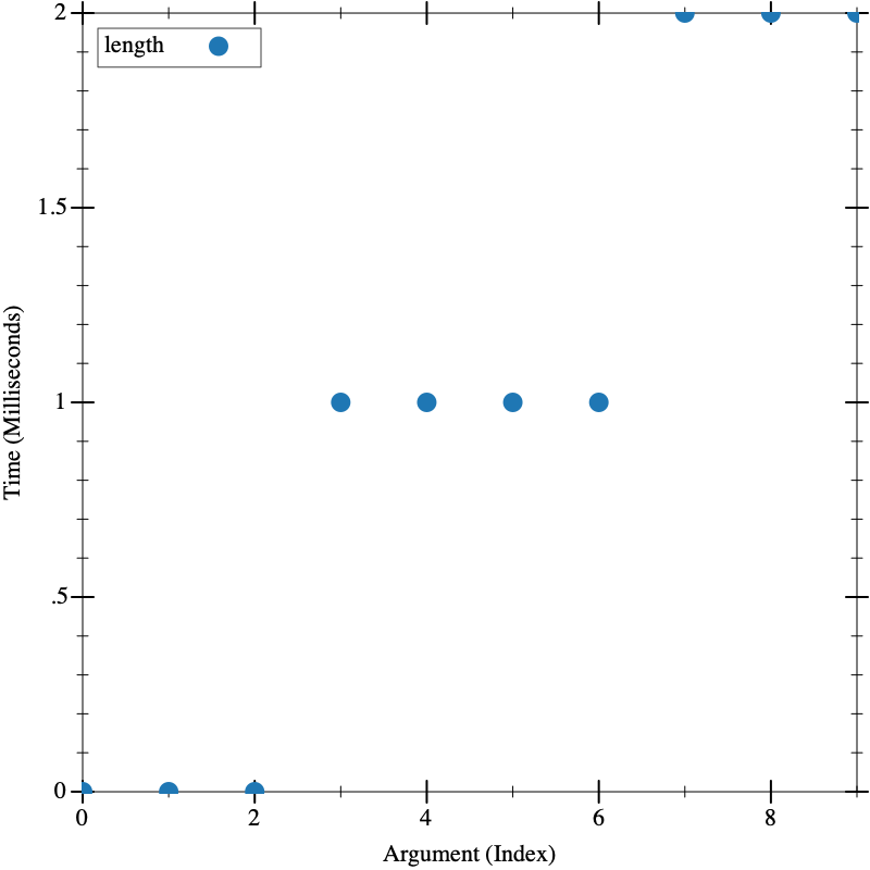
(visualize (build-list 10 (lambda (n) (build-list (* 100000 n) (lambda (_) 1))))            length)

The first thing we notice is that the graph is stepped. If you look at the Y axis, you see time, and notice that the first few arguments took 0ms, the next several took 1ms, and the last few took 2ms. This is an indication that our inputs are just not big enough. Since Racket 8.11 can take the length of a list with 1 million elements in ~2ms (on an Apple M2 chip), the intermediates (100,000, 200,000, etc) really aren’t going to give us enough granularity.

If we bump the size up by 10, we get different results:

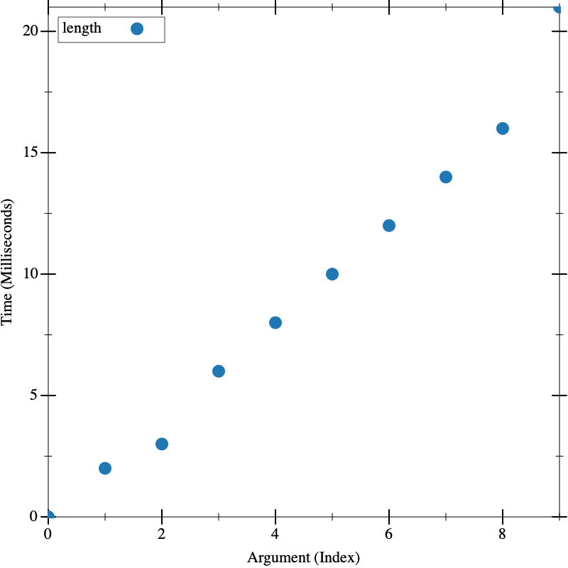
(visualize (build-list 10 (lambda (n) (build-list (* 1000000 n) (lambda (_) 1))))            length)

Now we can see the time going up linearly with the input size.

Which is faster

We can also use visualize to figure out which, of several implementations, is faster.

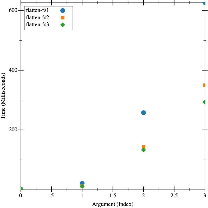
Consider the tree flattening code from Lecture 28: Concurrency Lab. Here we’ve written three different implementations. First, we have the implementation provided in Lecture 28: Concurrency Lab. Then we made a version that accumulates a path as it goes down the tree, rather than reconstructing it on the way back up. But accumulating makes us do lots of append operations, so we have a third where we instead accumulate a reversed path and then do a single reverse to correct it at the leaves.

Which do you think will be faster?

(struct file (name contents) #:transparent)

(struct directory (name elements) #:transparent)

(struct path [elts] #:transparent)

(define FS0 (directory "D" (list (file "e" "yow!")                                  (file "f" "eek"))))

(define FS1 (directory "A" (list (file "b" "hello there")                                  (file "c" "goodbye")                                  FS0                                  (directory "G" (list)))))

(define (mk-full-fs depth)   (if (zero? depth)       (file "a" "")       (directory "d"                  (build-list depth                              (lambda (_)                                (mk-full-fs (sub1 depth)))))))

(define FS (list (mk-full-fs 7)                  (mk-full-fs 8)                  (mk-full-fs 9)                  (directory "x"                             (list (mk-full-fs 9)                                   (mk-full-fs 9)))))

(define (flatten-fs1 fs)   (cond [(file? fs) (list (file (path (list (file-name fs))) (file-contents fs)))]         [(directory? fs)          (apply append                 (map (lambda (de)                        (map (lambda (x)                               (file                                (path                                 (cons (directory-name fs)                                       (path-elts (file-name x))))                                (file-contents x)))                             (flatten-fs1 de)))                      (directory-elements fs)))]))

(define (flatten-fs2 fs)   (local ((define (flatten-fs-acc pth fs)             (cond [(file? fs) (list (file (path (append pth (list (file-name fs)))) (file-contents fs)))]                   [(directory? fs)                    (apply append                           (map (lambda (de)                                  (flatten-fs-acc (append pth (list (directory-name fs)))                                                  de))                                (directory-elements fs)))])))     (flatten-fs-acc '() fs)))

(define (flatten-fs3 fs)   (local ((define (flatten-fs-acc rev-pth fs)             (cond [(file? fs) (list (file (path (reverse (cons (file-name fs) rev-pth))) (file-contents fs)))]                   [(directory? fs)                    (apply append                           (map (lambda (de)                                  (flatten-fs-acc (cons (directory-name fs)                                                        rev-pth)                                                  de))                                (directory-elements fs)))])))     (flatten-fs-acc '() fs)))

(visualize FS flatten-fs1 flatten-fs2 flatten-fs3)

Exercise:

Consider the following functions, that all sort lists of numbers:

; (: isort< (-> (List Number) (List Number)))

(define (isort< lon)   (local ((define (insert n slon)   (cond [(empty? slon) (list n)]         [else          (if (< n (first slon))              (cons n slon)              (cons (first slon) (insert n (rest slon))))])))     (cond [(empty? lon) '()]           [else (insert (first lon) (isort< (rest lon)))])))

; (: qsort< (-> (List Number) (List Number)))

(define (qsort< lon)   (cond     [(empty? lon) empty]     [(empty? (rest lon)) lon]     [(cons? lon)      (local ((define pivot (first lon))              (define smallers (filter (lambda (x) (< x pivot)) lon))              (define equals (filter (lambda (x) (= x pivot)) lon))              (define biggers (filter (lambda (x) (> x pivot)) lon)))        (append (qsort< smallers) equals (qsort< biggers)))]))

; (: msort< (-> (List Number) (List Number)))

(define (msort< lon)   (local ((define (merge lon1 lon2)             (cond [(and (empty? lon1) (empty? lon2)) '()]                   [(and (empty? lon1) (cons? lon2)) lon2]                   [(and (cons? lon1) (empty? lon2)) lon1]                   [(and (cons? lon1) (cons? lon2))                    (cond [(< (first lon1) (first lon2))                           (cons (first lon1)                                 (merge (rest lon1) lon2))]                          [else                           (cons (first lon2)                                 (merge lon1 (rest lon2)))])]))           (define lenlon (length lon)))     (if (<= lenlon 1)         lon         (local ((define midpoint (quotient lenlon 2))                 (define (take n lon)                   (cond [(zero? n) empty]                         [(positive? n) (cons (first lon) (take (sub1 n) (rest lon)))]))                 (define (drop n lon)                   (cond [(zero? n) lon]                         [(positive? n) (drop (sub1 n) (rest lon))]))                 (define left (take midpoint lon))                 (define right (drop midpoint lon)))           (merge (msort< left)                  (msort< right))))))

Use the following helper:

(define (mk-list n)   (build-list n (lambda (_) (random 10000))))

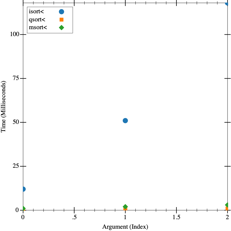
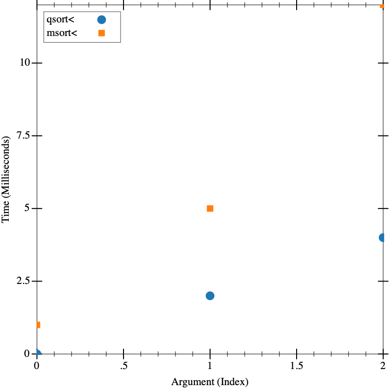
To investigate the performance of the three functions. Which is the fastest? You may need to do several rounds of testing, first with all three, then with the top two.

(visualize (list (mk-list 1000) (mk-list 2000) (mk-list 3000))            isort<            qsort<            msort<)

(visualize (list (mk-list 1000) (mk-list 5000) (mk-list 10000))            qsort<            msort<)