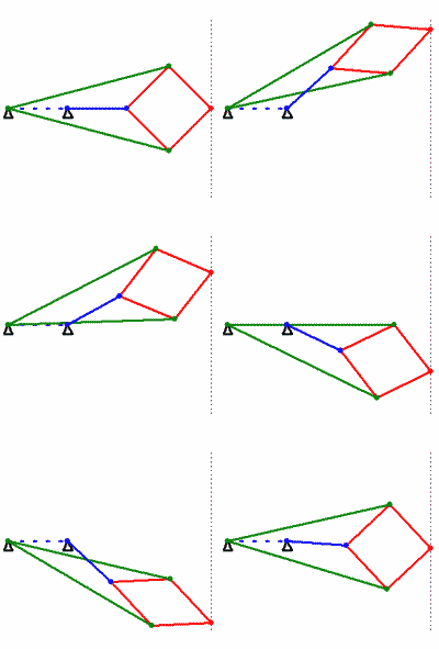
- Install the free version 1.4 of the dynamic geometry software Cinderella. On Windows you may have better luck using the “with JVM” download, and on Windows 7 you may need to right click on the installer executable in Windows Explorer and set the compatibility mode to Windows NT. Please use only version 1.4 for this assignment.
- Familiarize yourself with the Cinderella manual (this is for the later version 2, which adds physics and scripting features, but the documentation for the core dynamic geometry functionality still applies to 1.4). In particular, you will find the documentation for General Operations and Operations for Elementary Geometry useful.
- Follow this tutorial to construct a 4-bar linkage in Cinderella (the fixed distance between the first and last “anchor” points acts as a fourth bar). Save your work, and include the resulting
.cdyfile with your hand-in. - Construct a model of the Peaucellier-Lipkin linkage in Cinderella. Your model should have line segments corresponding to the red, green, and blue segments in the animation above (you can set the color of objects easily in Cinderella). Design your model so that you are free to change the angle of the blue segment (possibly by dragging one of its endpoints). Save your work, and include the resulting
.cdyfile with your hand-in. - Use Cinderella to generate the locus of the position of the rightmost point on the linkage as a function of the motion of the blue segment (or at least, as a function of its moving endpoint).
- The above locus should look like a straight line, which is the point (pun?) of the linkage. However, “looking” like a line does not prove that the motion is in fact a straight line. Add a construction for an actual line
 corresponding to the dotted line in the above animation (
 should also end up on top of the generated locus). The construction for
  must not depend on the blue segment (or its moving endpoint). Use Cinderella’s probabilistic theorem prover to verify that the rightmost point on the Peaucellier-Lipkin linkage actually does travel along a straight line. (Open the “information window” by the menu function “Views->Information Window” and look for a message to appear when you add the constructed line.) Save your work, and include the resulting
 .cdyfile with your hand-in. (Note: you should hand in a total of 3.cdyfiles, one for part c, one for part d, and one for part f. These count as “code”, so you may work with a partner on this problem.)
We have studied a variety of parameterizations for 3D rotation, including rotation matrices, Euler angles, unit quaternions, and the exponential map. In general it is possible to convert among them; for example, a given unit quaternion ![]() it is possible to calculate an equivalent
it is possible to calculate an equivalent ![]() orthogonal rotation matrix
orthogonal rotation matrix ![]() . Such conversions can be viewed as mathematical mappings from
. Such conversions can be viewed as mathematical mappings from ![]() to
to ![]() where
where ![]() is the size of the input parameterization and
is the size of the input parameterization and ![]() is the size of the output parameterization. For example
is the size of the output parameterization. For example ![]() and
and ![]() in the mapping from
in the mapping from ![]() to
to ![]() .
.
It is also true that the forward kinematics of a serial-chain robot, for example the three-link manipulator developed in the beginning of Selig Chapter 4, is a mapping from some ![]() dimensional input space to some
dimensional input space to some ![]() dimensional output space. In this case,
dimensional output space. In this case, ![]() equals the number of degrees of freedom in the robot joints (if every joint has only one degree of freedom, such as one rotation, then
equals the number of degrees of freedom in the robot joints (if every joint has only one degree of freedom, such as one rotation, then ![]() is simply the number of joints), and the input space is called the joint space. We use
is simply the number of joints), and the input space is called the joint space. We use ![]() to represent a vector in this space. And typically
to represent a vector in this space. And typically ![]() is either 2 or 3 for a planar robot, controlling the
is either 2 or 3 for a planar robot, controlling the ![]() position of the end-effector and possibly also its orientation (similarly,
position of the end-effector and possibly also its orientation (similarly, ![]() is typically either 3 or 6 for a spatial robot). The output space is called the task space, and we use
is typically either 3 or 6 for a spatial robot). The output space is called the task space, and we use ![]() to represent a vector in it. The forward kinematic mapping can thus be written as a function that takes an
to represent a vector in it. The forward kinematic mapping can thus be written as a function that takes an ![]() -vector input and produces an
-vector input and produces an ![]() -vector output:
-vector output: ![]()
We have further studied that the Jacobian is defined for the kinematic mapping ![]() as an
as an ![]() matrix of partial derivatives. The entry in this matrix at row
matrix of partial derivatives. The entry in this matrix at row ![]() col
col ![]() is
is ![]() .
.
In fact, Jacobians are defined in the same manner not just for robot kinematics, but for any differentiable mapping from ![]() to
to ![]() . A “Jacobian” is just the multidimensional equivalent of a derivative. It turns out that the mappings that represent conversions among rotation parameterizations are differentiable, and in this problem you will derive symbolic expressions for some of their Jacobians.
. A “Jacobian” is just the multidimensional equivalent of a derivative. It turns out that the mappings that represent conversions among rotation parameterizations are differentiable, and in this problem you will derive symbolic expressions for some of their Jacobians.
- On the second-from-last page his famous SIGGRAPH’85 paper, Shoemake gives a formula for converting a unit quaternion
 to a
to a  orthogonal rotation matrix
  . We may consider this formula to be a mapping
  . Derive symbolic expressions for the four partial derivatives
  ,
,  ,
,  ,
,  of this mapping. Write each as a
  matrix, with each entry an expression involving only
  . The Jacobian
  of
of  can be considered a
  matrix where the first column consists of the 9 entries of
  “unraveled”, the second column consists of the 9 entries of
  , etc.
 - Grassia’s paper centers on the exponential map
 where
where  and
and  . What are the dimensions of the Jacobian
  of this map? Derive expressions for all its components in terms of the quantities
  . Show your work in the derivation (if you read carefully, you will note that Grassia gives the final answers; you may ignore the case that
  is near zero).
 - For what set of surfaces
 do all exponential map vectors
  correspond to the same rotation? Note that a surface must be two-dimensional.
 - Finally, consider the composite mapping
 . The input is a 3-dimensional exponential map vector, and the output is a
  orthogonal rotation matrix. What are the dimensions of the Jacobian
  of this mapping? Give a short formula for computing it, using the results of parts a and b.
Using a programming environment of your choice (*), write a program that graphically displays a simulation of an ![]() -link planar revolute chain robot, i.e. a generalization of the three-link robot shown in figure 4.1 of the Selig reading. All links should have equal length, and the number of links
-link planar revolute chain robot, i.e. a generalization of the three-link robot shown in figure 4.1 of the Selig reading. All links should have equal length, and the number of links ![]() should be settable when the program is invoked (i.e. without requiring a re-compile). Set up the scale of your graphics output so that
should be settable when the program is invoked (i.e. without requiring a re-compile). Set up the scale of your graphics output so that ![]() in the range 1 to 10 are clearly shown in the window. The initial pose of the robot should be “straight out”, like the home position in Selig’s development. This should correspond to setting all the joint rotations to zero.
in the range 1 to 10 are clearly shown in the window. The initial pose of the robot should be “straight out”, like the home position in Selig’s development. This should correspond to setting all the joint rotations to zero.
(*) The only limitation on programming environment is that the course staff needs to be able to compile (if applicable) and run your program for grading purposes (note that it is not sufficient to simply supply both the source code and a pre-compiled executable—if you use a compiled language, we need to be able to re-compile your code). This mainly limits you to using freely-available programming environments, though we do have Matlab. Please resolve any questions you may have about this requirement with the course staff prior to beginning your work.
- Implement a feature to control the simulation by forward kinematics, i.e., setting joint angles. One way would be to allow the user to click on a joint to select it, then use the keyboard or mouse to set its angle. The specific design is up to you, but you must document how to use it in the README file that accompanies your hand-in. It should be possible to set every joint to its own angle, independent of the setting of other joints.
Implement a second feature to control the simulation by inverse kinematics. You should be able to click and drag on the end effector (the outer tip of the last segment of the robot), and the program should dynamically compute joint angles to make the end effector follow the mouse. Again, the exact design is up to you, including the choice of IK algorithm, but please document the design (and how to use it) your README. Reasonable options include the Jacobian transpose, pseudoinverse, and damped least squares methods as presented in the Buss reading. If you do choose to use any of these methods, please state so in your README.
You may also find the method to compute the Jacobian on page 5 of the Buss reading to be very handy.
When
 there are more joints than needed to make the end effector follow the mouse, provided the mouse point is reachable at all (i.e. provided it is no further than
  from the first joint, where
  is the link length). In such cases the robot is called redundant with respect to the task, and there are an infinite number of postures the robot could take that all satisfy the task. Make sure the IK method you choose works for these cases. In particular, analytical IK (solving the equations in closed form, as Selig later does for the two-link case) generally does not work for redundant robots.
Speed is important; it is not hard to implement IK that is not perceptibly “slow” for serial chains of up to at least
 on modern desktop and laptop computers.

