- a diff drive robot can have any position and orientation in the plane
- three degrees of freedom, which can be defined as
- two perpendicular translation components
 that give the location of an identified point on the robot relative to an identified point in the environment
- the relative angle
 between an identified vector on the robot and an identified vector in the environment
- together, we can call the position and orientation of the robot its pose
- define a world frame with basis (i.e. perpendicular unit vectors in axis directions)

and origin

- define a robot frame that moves with the robot. Put the origin
 of robot frame at the point on the ground midway between the contact points of the two wheels. Define the robot frame basis
 so that
 points forward on the robot and
 points to the robot’s left.
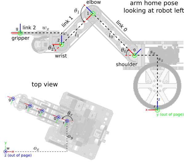
- the image below shows the robot frame, labeled “r”, and the world frame, labeled “w”, (ignore the arm frames for now)
- the actual numbers of
 measure where the robot currently is relative to world frame
-
is a point in world frame
-
and
are unit vectors in world frame
- 6 total numbers, but we only wanted 3
- actually not any choice of 6 numbers for
is allowed, because
and
must be perpendicular unit vectors


- these three constraints reduce the space of possible numeric assignments to
from 6 to 3 dimensions
- we can choose any
 and then set
 to denote the robot’s position
- we can then choose any
 and set
 to denote the robot’s

- this makes
the CCW angle from
 to
(measured in radians)
to
(measured in radians)
-
is also determined by
:
 (remember your trig identities?)
- in matrix form, the robot frame basis is thus

- those that have studied linear algebra will recognize that the constraints make this matrix orthogonal (it is also a rotation matrix)
- we can use
 to transform vectors from robot frame to world frame:

- for example, if
 is a unit vector pointing straight ahead with coordinates measured in robot frame

is the same vector but with coordinates measured in world frame (note in this case
 )
)
- to transform a point
 (i.e. a location) in robot frame to world frame, first consider
 to be a vector relative to
, transform it as above, and then add
:
to be a vector relative to
, transform it as above, and then add
:

- this can be made more convenient by defining a
 homogenous transformation matrix
 or, using
,
or, using
,

- then extend
 from
from
 to
to
 by appending a third homogenous coordinate equal to 1, and we can write the whole transformation from robot to world coordinates as a single matrix multiplication:

- what about going the other direction, i.e. transforming a vector or point from world to robot frame?
- since
is orthogonal, it is trivial to invert: the inverse of any orthogonal matrix is its transpose:

- we can then derive


- and


- putting the latter into homogenous form,
 with
with

Diff Drive: Forward Velocity Kinematics
- we want to drive the robot around!
- we can tell the motor drivers to supply power to the motors, which will make the left and right wheels independently rotate forward or backward at some rotational velocities
 (let these be measured in radians per second, and define them so that the robot moves forward when they are positive)
- but how fast does this make the robot move?
- this is a question of forward kinematics: we know the motions of the actuators; we want to predict the motion of the robot
- over a short time interval, the robot’s position
and orientation
will change a little
- in the limit as this time interval approaches zero, we can define
 as the robot’s translation velocity in world frame
 as the robot’s rotation velocity in world frame
- observe that in this limit, the constraints of the wheel interaction with the ground (the wheels cannot go directly sideways) imply that
 is parallel to
- so we can define a scalar robot translation speed
 where
where

- we can thus summarize the robot speed as the pair

- in robot frame:
- the translation velocity is


i.e. a vector pointing straight forward with magnitude
- the rotation velocity is still

- how are
determined as a function of
 ?
?
- at any instant, it is not hard to see that the robot speed is the average of the wheel speeds on the ground
 :
:

- what are
given
?
- remember that the length
 of a circular arc with radius
 and angle
 in radians is
 (derivation:
 ,
,
 ,
,
 )
)
- so

- finally we get


where
is the wheel radius
- to find
, notice that only the difference between the wheel speeds matters
- consider a moving coordinate frame with origin at the point of contact of the left wheel with the ground
- in this frame, the right wheel speed is

- let the distance between the wheels be

- then the point of contact of the right wheel on the ground moves along a circular arc in the moving frame, centered at the left wheel’s point of contact, with radius
- if the robot rotates by
 over a short time interval, the length of this arc will be

- the arc length is also
 , where
 is the time interval:


- the two key equations can be summarized in matrix form:

- Assume the robot drives at a constant linear speed
and angular speed
for a time interval
 . What trajectory will be driven? (Ans: an arc with radius
 , subtending angle
 , and with arc length
 .)
.)
Diff Drive: Inverse Velocity Kinematics
- it is also clearly going to be useful to calculate
given
- we can apply the analytic inverse of a
 matrix

to invert the
matrix in the final equation for the forward velocity kinematics:

- multiply both sides of the forward velocity kinematics equation by this and by
 to get

- done!
Diff Drive: Forward Position Kinematics
- TBD mention dead reckoning here
- if we assume the wheels do not slip on the ground, we should be able to keep track of the robot pose
 or simply
 in world frame, relative to its starting value
 , just by keeping track of the wheel rotations
- another way to put it is that, given the time histories, also called trajectories of
 as functions of time,
 from
from
 until “now” at time
 , we should be able to theoretically predict the corresponding pose trajectory
 from
until
from
until
- this process, which gives us an estimate of the robot’s position at any time, is called odometry
- note again that
is only known relative to
 ; in practice a very common approach is just to define world frame to coincide with robot frame at
- one way to get
is to take the derivative of
to get
 , then apply the forward velocity kinematics transformation above to get
 , and then integrate
- our development follows the nice writeup here
- starting with orientation, recall that we had derived

- this can be directly integrated to give

where

-
 if using the convention that the robot starts out aligned to world frame
- moving on to position, recall we had defined
 , where
is the world-frame robot velocity,
is the forward speed of the robot in robot frame, and
is a world-frame vector that points forward on the robot depending on its current orientation
, where
is the world-frame robot velocity,
is the forward speed of the robot in robot frame, and
is a world-frame vector that points forward on the robot depending on its current orientation
- we had also derived the relationship
- putting these three together gives

- if we assume that the wheel velocities
remain constant, then (using integration by substitution) we can integrate this to give

where

-
 if using the convention that the robot starts out aligned to world frame
- This equation can also be derived by a purely geometric analysis, without calculus — the constant velocity assumption means that over any time interval
the robot will travel along a well-defined arc path.
- our assumption that the wheel velocities remain constant will be violated, of course
- but over short enough time intervals, the violation is minimized
- this suggests an approach to use these equations for incremental odometry
- adapt the equation for
 to
to

where
 are the changes in the two wheel angles from the beginning to the end of the time interval
- and adapt the equation for
 to
to

where
 is the estimated robot orientation at the start of the interval
- be careful: what happens to this equation when
approaches zero? It becomes the indeterminate form

- in that case l’Hôpital’s rule says to replace each component with the deriviative of the numerator over the derivative of the denominator
- the result is the same as the point and shoot approximation below, with

- then update the odometry estimate by

where
 is the estimated robot position at the start of the interval, and
 and
and
 are the updated estimates of the robot position and orientation at the end of the interval
- sometimes people take an even simpler approach and model all the rotation change to happen instantaneously at the start of the interval
- the equation for
stays the same
- now estimate
 as
as

- this is sometimes called the point and shoot approximation
- no divide by zero problem when

Diff Drive: Inverse Position Kinematics
- One way to frame position inverse kinematics is to find wheel rotation trajectories
corresponding to a given state trajectory
.
- We could follow a similar approach as above: differentiate
 to get
, apply the inverse velocity kinematics transformation, and then integrate.
to get
, apply the inverse velocity kinematics transformation, and then integrate.
- However this is rarely done. More frequently, a variation of the problem is considered where only the start and final poses are given.
- The position IK problem is not well defined then, because there are infinitely many trajectories to get from one pose to any other.
- We can seek trajectories that minimize certain quantities of interest, for example the total travel time, or the total amount of wheel rotation. Perhaps surprisingly, even these seemingly straightforward problems have been subjects of recent research.
- Other simple approaches include the turn-drive-turn strategy:
- turn in place to face the goal location
- drive to the goal location
- turn in plaece to the goal orientation
- Or driving in two equal-radius arcs which meet at a common tangent, as demonstrated in this matlab script.
- All of this assumes that there are no obstacles in the environment. It is usually more practical to consider obstacles, in which case the problem is called (local or global) path planning or navigation.
