Computer Graphics (CS 4300) 2010S: Lecture 6

Today

• alpha blending
• image compression
• image scaling

Alpha Blending

• how to rasterize transparent objects?
  • if object is totally transparent, then just do nothing
  • i.e. let the “background” show through unmodified
• for a partially transparent, or translucent object, one common approach is alpha blending
• idea: for each pixel, combine the underlying background color with the foreground color , i.e. the color of the object itself at that pixel, to produce the overall pixel color according to the formula
• the parameter sets the amount of transparency
  • shows only the object
  • shows only the background
  • shows half object and half background
  • etc.
• this is an example of linear interpolation
• the process of combining a background image with a foreground image is called compositing
• can chain the process to composite many images on top of each other
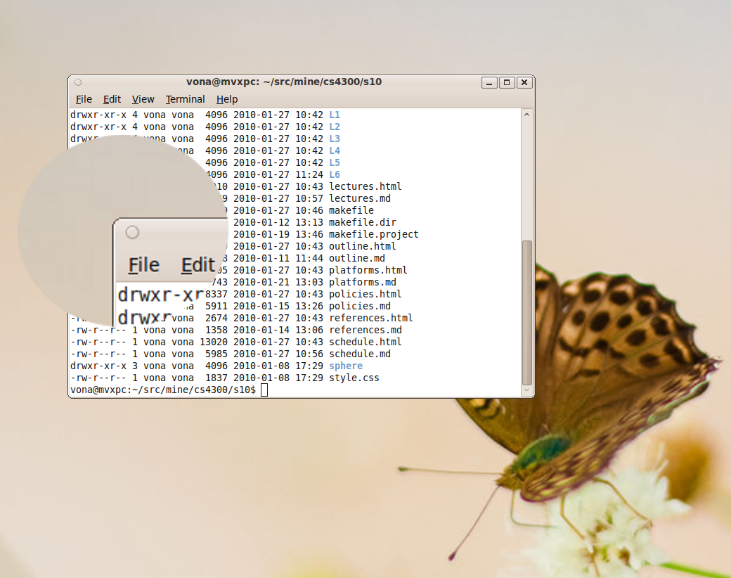
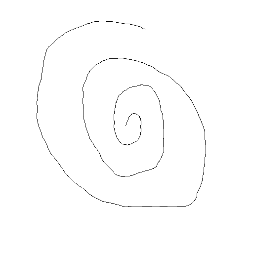
• this image shows a terminal window composited with onto a desktop background
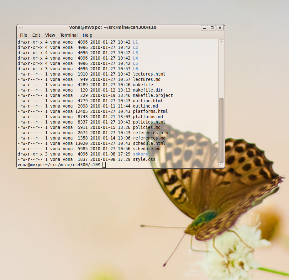
• this image shows a terminal window composited with onto a desktop background
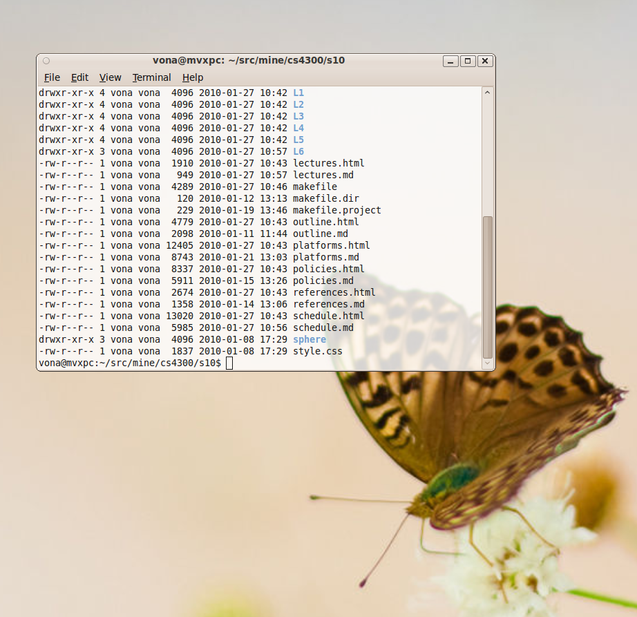
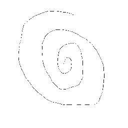
• this image shows a terminal window composited with onto a desktop background
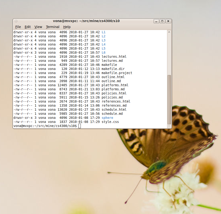
• sometimes a single is specified for an entire object (e.g. could be considered a line attribute)
• for a raster, is commonly treated as a separate color channel, along with (typically) R, G, and B
  • thus, an RGB image with an added alpha channel is sometimes referred to as an RGBA image
  • this allows setting a different value for each pixel in the raster
  • often, a similar number of bits is allocated for the alpha channel as for the other color components
  • conveniently, adding an 8 bit alpha channel to a 24 bit RGB image results in an image with 32 bits per pixel
  • 8 bits is not enough to store an IEEE floating point single or double precision number, so instead alpha is represented as an integer where the actual fractional alpha value is computed as
  • most modern microprocessors are especially fast at moving around 32 bit “words”
  • even if 8 bits are available, sometimes the alpha channel is used only as a binary image
    • i.e. the (floating point) alpha value for any given pixel is either 0.0 (show background only) or 1.0 (show foreground only)
    • this produces a binary image mask
    • one use is to allow non-rectangular windows

Image Compression

• rasters take up a lot of memory!
  • example: 640x480x3 BPP (Bytes Per Pixel): 921,600 bytes, or nearly 1MB
  • example: 1600x1200x4 BPP: 7,680,000 bytes, or a bit over 7MB
• usually, when a raster has to actually be displayed on the screen, we do need to keep the whole thing in memory
• but for storing and transferring images, we can usually do better by compressing the data
• an image compression algorithm starts with the original raster, and produces a stream of bytes which describes the image, ideally so that the length of that stream of bytes is significantly smaller than the original raster
• an image decompression algorithm does the opposite
• today, two compression algorithms are very common in practice: Portable Network Graphics (PNG) and the Joint Photographic Experts Group method (JPEG)
  • actually, these are not only compression and decompression algorithms, but also standards for the specific layout of the associated byte streams
• we will not cover the full details of either algorithm, but only cover the broad strokes
  • implementing good image compressors and decompressors that are both correct and fast is a significant undertaking
  • this is a case where you want to take advantage of the libraries and APIs available to you as much as possible
  • but it’s still important to basically understand what they’re doing, so that you can set their parameters, or even just make a simple decision like…
• which is better, PNG or JPEG?
  • PNG supports both color, greyscale, and indexed images, and allows inclusion of an alpha channel
  • JPEG supports color and greyscale images, but not indexed, and does not allow inclusion of an alpha channel
  • but most importantly, PNG is lossless, while JPEG is lossy:
    
• PNG is a lossless compression technique: the raster that results from decoompression is guaranteed to be exactly the same as the original
  • often a compression ratio of 5:1 to 10:1 is still achieved, because image data is typically redundant
    • e.g. there are often areas filled with a single color
  • this is particularly true for computer generated images, like line drawings, cartoon graphics, and user-interface graphics, that do not depict real-world scenes
  • these are also the kinds of scenes for which JPEG compression is poorly suited, as we will see later
  • the basic process of PNG compression takes two stages
    1. first, a pre-compression prediction filter is applied to the image
    2. then, a standard general purpose lossless compression algorithm called DEFLATE is applied to the raster, treated as a linear array of bytes
  • DEFLATE is the same algorithm used in the common zlib compression library, which is what implements gzip, a variant of ZIP
  • we will not cover DEFLATE, but we will look at the first step, the prediction filter
  • one problem with DEFLATE is that by treating a raster as a linear sequence of bytes, correlations from one row to the next may be lost
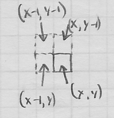
  • the PNG prediction filter essentially replaces the value of each color component of a pixel at with a difference between the actual value in the original image and a value that would be predicted for that pixel based on the three pixels at , , and .
    
  • how is the prediction made? The compressor uses heruistics to select among a fixed set of five different options.
    • “none”—the predicted value is 0
    • “sub”—the predicted value is the value at
    • “up”—the predicted value is the value at
    • “average”—the predicted value is the average of the values at and
    • “paeth”—a bit more complex
  • the compressor selects one of these to use for each line of the raster
    • the whole line then uses the same method, but different lines may use different methods
    • a notation is put in the compressed bytestream so that the decompressor can “undo” the filter
• JPEG is a lossy compression algorithm: the raster that results from decoompression is not guaranteed to be exactly the same as the original
  • this often allows significantly more compression than PNG
  • some of the data is actually discarded
  • the idea is to try to prioritize so that the least perceptually significant data is discarded first
  • JPEG can achieve a compression ratio ranging from typically around 10:1 for high quality to 100:1 for low quality
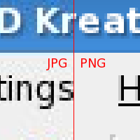
  • this image was specially constructed with increasing JPEG compression from left to right:
    
  • JPEG compression is well-suited for scenes where colors change contagiously, without sharp edges
  • in particular, real-world scenes captured with cameras often compress well with JPEG
  • computer-generated line drawings and other art will become blurred at sharp edges
  • the basic process for JPEG compression takes five steps
    1. original RGB data is converted to a color space called YCbCr. We did not study this; but it is another space where the brightness or luminance (Y) is separated from the color information, in this case Cb and Cr.
    2. because the eye is less sensitive to color details than it is to intensity, Cb and Cr are typically thrown out for half of the pixels
    3. for each block of 8x8 pixels, a discrete cosine transform is applied (see below)
    4. the DCT is lossless, but puts the data into a frequency domain form where we can more easily discard perceptually less significant information. In particular, rapid high frequency variations are less noticeable than slower changes. So some of the bits are discarded for the high frequency components. This is an instance of quantization.
    5. the resulting bitstream is losslessly compressed, in this case with the version of Huffman encoding
    • so what is DCT? we will not cover the math, but the intuition is actually similar to our discussion in L5 of how the human eye decomposes an arbitrary spectral histogram into three color components
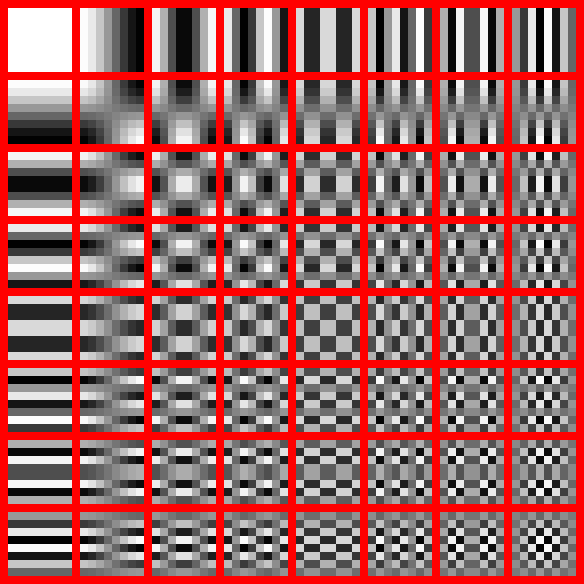
    • in this case, the DCT algorithm decomposes a block of 8x8 pixel color component values (separate DCT are done for Y, Cb, and Cr) into a weighted sum of the following basis functions
      
    • whereas for color perception, the mapping was not 1:1—aliasing could occur where the eye perceives two different incident spectra as the same color—in this case the basis functions are carefully constructed so that the mapping is 1:1
      • observe that the original 8x8 block of pixel color components was stored in e.g. bits
      • if 8 bits are used to represent the relative weight of each of the above basis functions, then the DCT result will again be 512 bits
      • this gives an intuition, the actual proof (and the way to compute the DCT) depends on math involving the Fourier Transform
      • so DCT conversion is itself lossless, but it is the quantization step where some of the bits for the weights for higher-frequency basis functions are discarded

Image Scaling

• very frequently, we would like to change the dimensions of a raster
• what does this mean?
• one thing we sometimes want is to crop an image
  • this is easy: just discard the rows above and below the desired subframe, and then discard the columns to its left and right
• more commonly, we would like the resulting raster to appear similar to the original, but just scaled up or down (i.e. zoomed in or out)
• one method is called decimation or pixel dropping
• this is fast to implement, but the results often do not look very good
  
  
• we can do better by again remembering that “a pixel is not a little square”
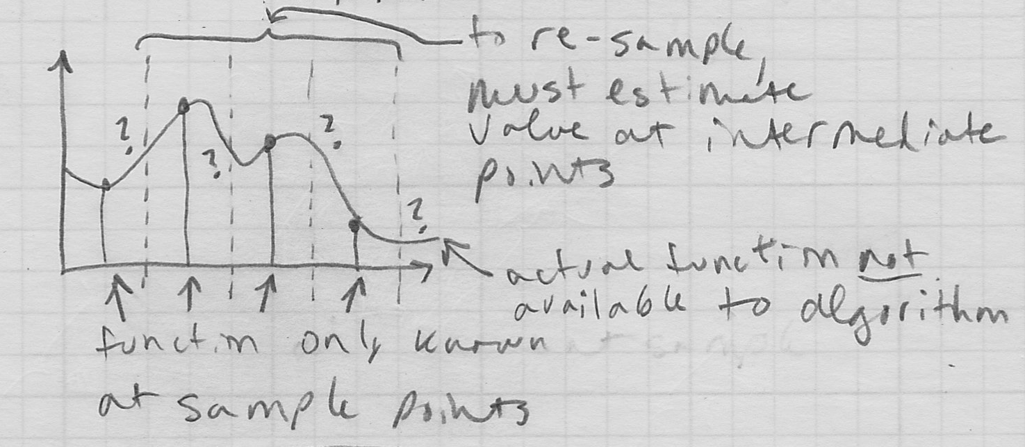
• to rescale the image, we should really resample it
  • diagram (1D)
    
• this will mean that we will somehow need to answer the question: what is the value of the image at a sample location between the original pixels?
• one way to think about this is that we need to reconstruct a version of what the original continuous domain image would have been, so that we can take new samples of it
• since all we have are the original samples, we will essentially have to “make up” the continuous image in-between them
• rather than getting crazy, generally we will make these in-between locations some kind of weighted average of neighboring samples
• there are various ways to do this: in GIMP or Photoshop one can typically choose between at least linear and cubic interpolation
• linear interpolation works like this (1D)
  • given the original samples ,
  • a desired resample location, a real (or floating point) number, ,
  • a filter radius ,
  • the new sample is computed as
    
  • this is a “tent function” with peak
    
    

Next Time

• graphical user interfaces; windowing toolkits; programming models for interactive graphics
• reading on website

this page subject to change  |  last updated Mon Apr 19 13:06:56 EDT 2010  |  course homepage