18 Homework 11B
Due:
Thursday, 3/28 at 9PM
This assignment is SOLO, and entirely AUTOGRADED.
What to Download:
Please start with this file, filling in where appropriate, and submit your homework to the HW11B assignment on Gradescope. This page has additional information, and allows us to format things nicely.
18.1 IMPORTANT NOTE
Since LSL does some things that make performance testing a little more difficult, for this assignment, we are using Racket instead. Not only is Racket a lot faster, it has a lot more "normal" performance characteristics.
We are using a library, lsl/performance, provided by LSL, to measure & graph the performance of functions.
18.2 Performance Testing
Technically, since we are measuring average performance, we are measuring big-θ, which is average case complexity, rather than big-O, which is worst case complexity, but for the problems we are looking at, which do not involve randomization, the distinction shouldn’t matter.
In each problem, you’re asked to move the function down a complexity class. i.e., in the list below, if you measure the function to perform at, e.g., O(n^2) (quadratic), then your task in to change it so that the code behaves as O(n) (i.e., linear), but O(1) (constant) would be fine as well. One important note: if you only test the functions on very small inputs, they may look constant when they are not. Since every problem can be moved down, none of them start out constant, but beware of doing inadequate measurement.
O(1) < O(n) < O(n^2) < O(2^n)
Note that there are many other complexities that fit it between these (e.g., O(n*log(n))), but distinguishing them from the others via a small enough number of samples might be hard, so we are simplifying (and, e.g., we’d consider O(n*log(n)) to look linear, as it often essentially behaves).
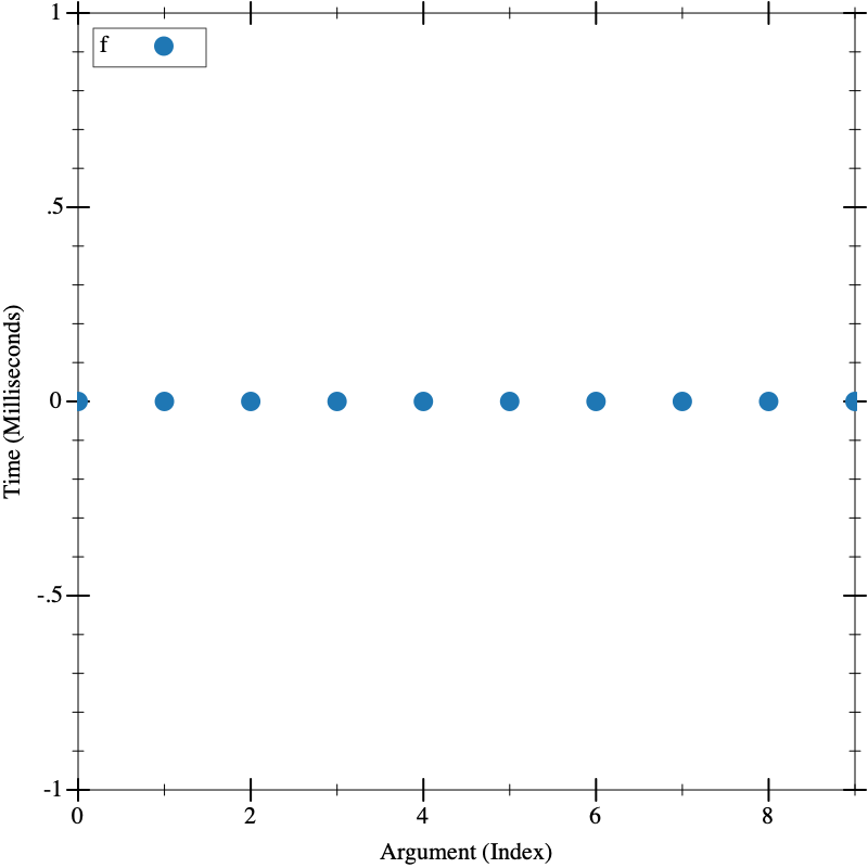
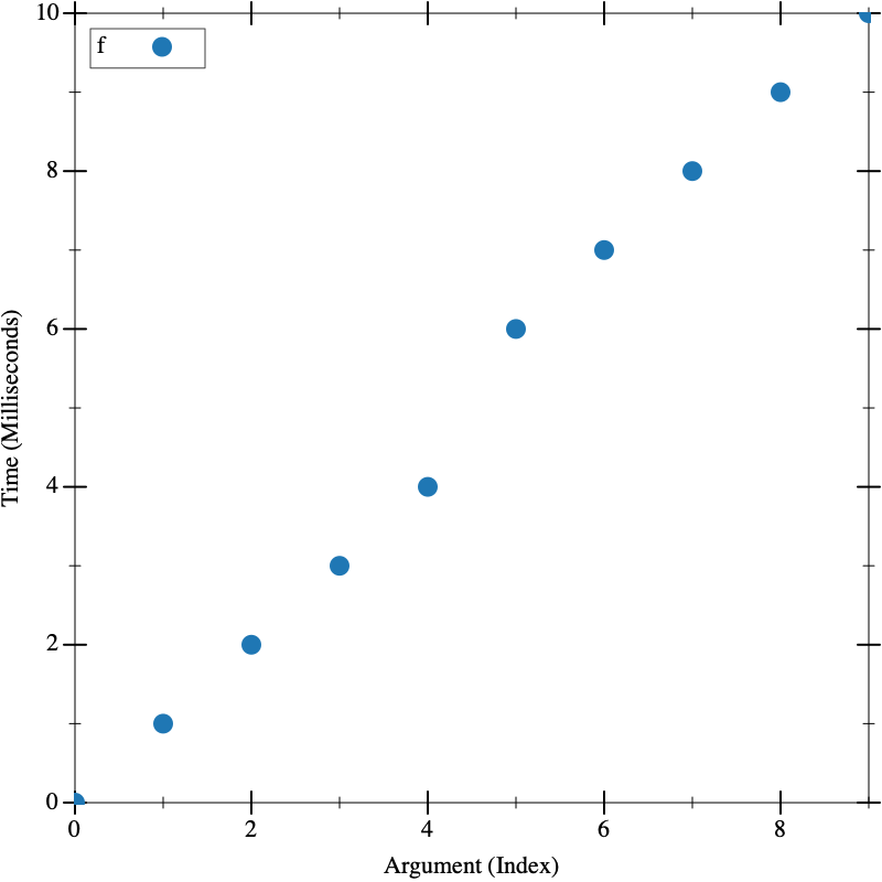
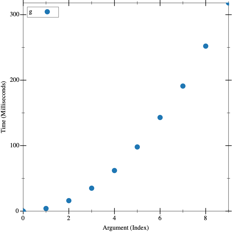
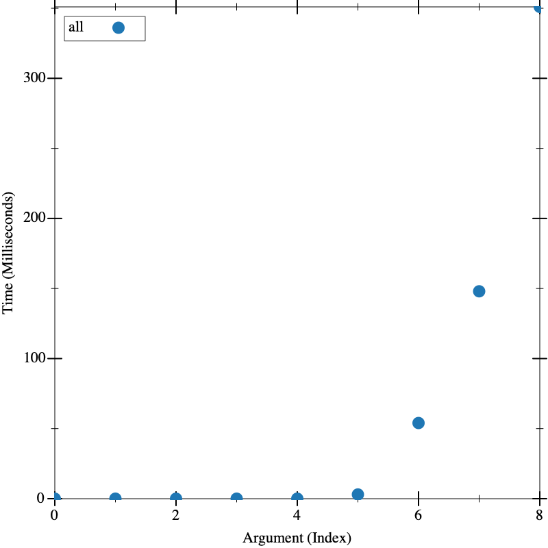
For reference when trying to understand the graphs produced by visualize, here are examples of simple graphs for each of the complexities:
(require lsl/performance)
O(1)
(define (f _) 1) (visualize (build-list 10 (lambda (n) (* n 1000))) f)
O(n)
(define (f n) (if (zero? n) 1 (f (sub1 n)))) (visualize (build-list 10 (lambda (n) (* n 700000))) f)
O(n^2)
(define (g n) (local ((define (f n) (if (zero? n) #t (f (sub1 n)))) (define (gl k) (if (zero? k) #t (and (f n) (gl (sub1 k)))))) (gl n))) (visualize (build-list 10 (lambda (n) (* n 2000))) g)
O(2^n)
(define (all n) (local ((define (all-local n) (cond [(zero? n) '(())] [else (let ([xs (all-local (sub1 n))]) (append (map (λ (x) (cons 1 x)) xs) (map (λ (x) (cons 0 x)) xs)))]))) (map reverse (all-local n)))) ; Going up by 3, but gets so fast towards end, showing intermediates (visualize '(0 3 6 9 12 15 18 19 20) all)
18.3 Problem 1
Consider the following function. Investigate it using visualize, figuring out appropriate inputs to pass to it to discover the time complexity (one of the four above), and then modify the code to shift it to a lower complexity class.
| (define (min-list l) |
| (if (empty? l) |
| #f |
| (if (or (boolean? (min-list (rest l))) |
| (< (first l) (min-list (rest l)))) |
| (first l) |
| (min-list (rest l))))) |
18.4 Problem 2
Consider the following function. Investigate it using visualize, figuring out appropriate inputs to pass to it to discover the time complexity (one of the four above), and then modify the code to shift it to a lower complexity class.
| (define (maybe-second l) |
| (if (>= (length l) 2) |
| (first (rest l)) |
| #f)) |
18.5 Problem 3
Consider the following function. Investigate it using visualize, figuring out appropriate inputs to pass to it to discover the time complexity (one of the four above), and then modify the code to shift it to a lower complexity class.
| (define (list-reverse l) |
| (cond [(empty? l) empty] |
| [(cons? l) (append (list-reverse (rest l)) (list (first l)))])) |
NOTE: you may not use the built-in reverse function.
18.6 Problem 4
Consider the following function. Investigate it using visualize, figuring out appropriate inputs to pass to it to discover the time complexity (one of the four above), and then modify the code to shift it to a lower complexity class.
| (define (fib n) |
| (cond [(<= n 1) 1] |
| [else (+ (fib (- n 1)) (fib (- n 2)))])) |


