Assignment 10: Mazes of twisty passages...no two alike!
Goals: Practice working with graphs and graph algorithms by designing mazes using Kruskal’s algorithm, and solving them using either breadth- or depth-first searches.
import java.util.ArrayList; import tester.*; import javalib.impworld.*; import java.awt.Color; import javalib.worldimages.*;
Make sure you do not name any of your files World.java, or else the autograder will not be able to compile your code.
As with homework 9, you will submit this project twice. For Part 1 you must have completed the tasks of building random mazes and drawing them. For Part 2 you must complete the remaining tasks of solving mazes (both depth- and breadth-first),
and any additional features or extra credit you attempt.
As with homework 9, extra credit will only count if they are convincingly and
thoroughly tested, and if the rest of the assignment is completed equally
thoroughly —
Part 1 Due: Thursday, April 13th at 9:00pm. (building and drawing random mazes)
Part 2 Due: Wednesday, April 19th at 9:00pm. (solving with both depth- and breadth-first and the rest of the requirements listed below, plus any additional features or extra credit)
In class, we have been discussing various algorithms for working with graphs, that require the use of several data structures working together. We have talked about general-purpose maze searching algorithms, like breadth- and depth-first searches, and we have talked about building minimum spanning trees on graphs.
To get a visual grasp of how these algorithms work, you are going to be building and solving mazes, like this one:

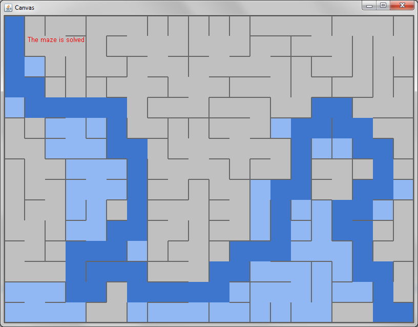
The mazes you construct should start in the upper-left corner (shown in green) and end in the lower-right corner (shown in purple). As you solve the mazes, you should color in the cells you have explored. Once you have reached the solution, you must backtrack the path from the end to the start, and draw it as well. A fully-solved maze might look like this:

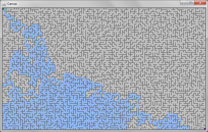
Your code must handle mazes of arbitrary sizes, up to at least 100x60:

In particular, your code must not crash with stack overflows...
10.1 Requirements
Construct random mazes using Kruskal’s algorithm and Union/Find (below)
Display the maze graphically and animate the search for the path.
Allow the user to choose one of two algorithms for finding the path: Breadth-First Search or Depth-First Search (below).
Provide an option for designing a new random maze.
Display the solution path connecting the start and end, once it’s found (either automatically or by the user).
Be sure to submit documentation for your code, so the graders know how to run and play your game. As always, be sure to test your code thoroughly.
Additionally, you may attempt bells and whistles for extra credit:
Provide an option to toggle the viewing of the visited paths.
Allow the user the ability to start a new maze without restarting the program.
Keep the score of wrong moves —
for either the automatic solutions or manual ones — and maybe keep statistics on which one of the two algorithms had fewer steps for each maze.
Allow the user to traverse the maze manually - using the keys to select the next move, preventing illegal moves and notifying the user of completion of the game.
In addition to animating the solution of the maze, also animate the construction of the maze: on each tick, show a single wall being knocked down.
(Tricky) Construct mazes with a bias in a particular direction —
a preference for horizontal or vertical corridors. (Hint: you might wish to play tricks with the edge weights here.) Hard! (But very cool) Instead of constructing a rectangular maze, try constructing a hexagonal one.
Spend careful thought planning ahead and designing your classes: if your design is too brittle, you’ll have a very hard time completing the algorithms. And as always, have fun!
10.2 Kruskal’s Algorithm for constructing Minimum Spanning Trees
A -----30------- B -----50------- F
 \             / |               /
  \           /  |              /
  50        35  40            50
    \       /    |            /
     \     /     |           /
      \   /      |          /
E --15-- C ---25-- D(E C 15) (C D 25) (A B 30) (B E 35) (B C 40) (F D 50) (A E 50) (B F 50)
At each step we remove the shortest edge from the list and add it to the spanning tree, provided we do not introduce a cycle. In practice, this may produce many trees during the execution of the algorithm (so in fact, the algorithm produces a spanning forest while it runs), but they will eventually merge into a single spanning tree at the completion of the algorithm.
while (we do not yet have a complete spanning tree) |
find the shortest edge that does not create a cycle |
and add it to the spanning tree |
Do Now!
Why can’t we have fewer edges? Why can’t we have more?
10.3 The Union/Find data structure
The goal of the union/find data structure is to allow us to take a set of items (such as nodes in a graph) and partition them into groups (such as nodes connected by spanning trees) in such a way that we can easily find whether two nodes are in the same group, and union two disjoint groups together. Intuitively, we accomplish this by naming each group by some representative element, and then two items can be checked for whether they are in the same group by checking if they have the same representative element.
10.3.1 Example
In class, we represented every node of the graph as a class with a String name field. (For this assignment, String names will be inconvenient; you will need to come up with some other uniquely-identifying feature of each cell in a maze that can serve the same role as a name.) Then the union-find data structure was a HashMap<String, String> that mapped (the name of) each node to (the name of) a node that it is connected to. Initially, every node name is mapped to itself, signifying that every node is its own representative element, or equivalently, that it is not connected to anything.
A -----30------- B -----50------- F
 \             / |               /
  \           /  |              /
  50        35  40            50
    \       /    |            /
     \     /     |           /
      \   /      |          /
E --15-- C ---25-- D Representatives, visually:
+---+---+---+---+---+---+ A B C D E F
Node: | A | B | C | D | E | F |
+---+---+---+---+---+---+
Link: | A | B | C | D | E | F |
+---+---+---+---+---+---+
Spanning tree so far:(E C 15) (C D 25) (A B 30) (B E 35) (B C 40) (F D 50) (A E 50) (B F 50)
                                      Representatives, visually:
        +---+---+---+---+---+---+     A     B     D     E     F
Node:   | A | B | C | D | E | F |                       ^
        +---+---+---+---+---+---+                       |
Link:   | A | B | E | D | E | F |                       C
        +---+---+---+---+---+---+

Spanning tree so far: (C E) Representatives, visually:
+---+---+---+---+---+---+ A B E F
Node: | A | B | C | D | E | F | ^
+---+---+---+---+---+---+ / \
Link: | A | B | E | E | E | F | C D
+---+---+---+---+---+---+
Spanning tree so far: (C D) (C E)Do Now!
Careful! Why must we union the representatives of two nodes, and not the nodes themselves?
                                      Representatives, visually:
        +---+---+---+---+---+---+     A     E     F
Node:   | A | B | C | D | E | F |     ^     ^
        +---+---+---+---+---+---+     |    / \
Link:   | A | A | E | E | E | F |     B   C   D
        +---+---+---+---+---+---+

Spanning tree so far:          (A B) (C D) (C E)
We now have three connected components: Nodes B and A form one of them, node F is a singleton, and nodes C, D, and E are in the third component.
                                      Representatives, visually:
        +---+---+---+---+---+---+       E     F
Node:   | A | B | C | D | E | F |       ^
        +---+---+---+---+---+---+      /|\
Link:   | E | A | E | E | E | F |     A C D
        +---+---+---+---+---+---+     ^
                                      |
                                      B

Spanning tree so far:          (A B) (B E) (C D) (C E)
We still have two components. When we try to add the edge (B C 40) to the graph, we notice that the representative for node C is the same as the representative for the node B. Therefore adding this edge would create a cycle, so we discard it.
                                      Representatives, visually:
        +---+---+---+---+---+---+       E
Node:   | A | B | C | D | E | F |       ^
        +---+---+---+---+---+---+      /|\
Link:   | E | A | E | E | E | D |     A C D
        +---+---+---+---+---+---+     ^   ^
                                      |   |
                                      B   F

Spanning tree so far:          (A B) (B E) (C D) (C E) (D F)
10.4 Putting the union/find data structure to work
HashMap<String, String> representatives; List<Edge> edgesInTree; List<Edge> worklist = all edges in graph, sorted by edge weights; initialize every node's representative to itself While(there's more than one tree) Pick the next cheapest edge of the graph: suppose it connects X and Y. If find(representatives, X) equals find(representatives, Y): discard this edge // they're already connected Else: Record this edge in edgesInTree union(representatives, find(representatives, X), find(representatives, Y)) Return the edgesInTree
There are additional heuristics for speeding this algorithm up in practice, and they make for a very efficient algorithm. Unfortunately, analyzing these heuristics is beyond the scope of this course, but you can look up the “path-compression” heuristic if you are curious.
Do Now!
Again, why must we only ever union two representatives, and not two arbitrary nodes?
10.5 Breadth- and depth-first search
HashMap<String, Edge> cameFromEdge; |
???<Node> worklist; // A Queue or a Stack, depending on the algorithm |
|
initialize the worklist to contain the starting node |
While(the worklist is not empty) |
Node next = the next item from the worklist |
If (next has already been processed) |
discard it |
Else If (next is the target): |
return reconstruct(cameFromEdge, next); |
Else: |
For each neighbor n of next: |
Add n to the worklist |
Record the edge (next->n) in the cameFromEdge map |