27 Lecture 27: Introduction to Big-O Analysis
When is one algorithm “better” than another?
27.1 Motivation
We’ve now seen several data structures that can be used to store collections of items: ILists, ArrayLists, BinaryTrees and binary search trees, and Deques. Primarily we have introduced each of these types to study some new pattern of object-oriented construction: interfaces and linked lists, indexed data structures, branching structures, and wrappers and sentinels. We’ve implemented many of the same algorithms for each data structure: inserting items, sorting items, finding items, mapping over items, etc. We might well start to wonder, is there anything in particular that could help us choose which of these structures to use, and when?
To guide this discussion, we’re going to focus for the next few lectures on various sorting algorithms, and analyze them to determine their characteristic performance. We choose sorting algorithms for several reasons: they are ubiquitous (almost every problem at some stage requires sorting data), they are intuitive (the goal is simply to put the data in order; how that happens is the interesting part!), they have widely varying performance, and they are fairly straightforward to analyze. The lessons learned here apply more broadly than merely to sorting; they can be used to help describe how any algorithm behaves, and even better, to help compare one algorithm to another in a meaningful way.
27.2 What to measure, and how?
Do Now!
What kinds of things should we look for, when looking for a “good” algorithm? (What does “good” even mean in this context?) Brainstorm several possibilities.
27.2.1 Adventures in time...
Suppose we have two sorting algorithms available to use for a particular problem. Both algorithms will
correctly sort a collection of numbers —
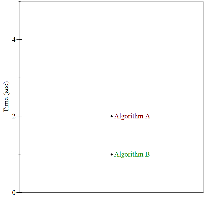
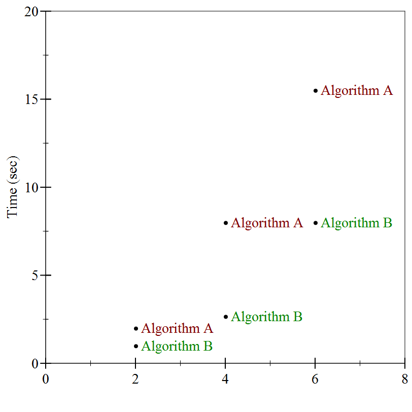
That hardly seems like enough information to decide which of the two algorithms performs better. We need to see how the two algorithms far on inputs of different sizes, to see how their performance changes as a function of input size. It turns out the particular input above was of size 2. When we run these two algorithms again on inputs of size 4, and again on inputs of size 6, we see
If we connect the dots, we see the following:
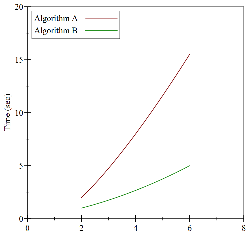
Still not much to go on, but it looks like Algorithm A is substantially slower than Algorithm B. Or is it? Let’s try substantially larger inputs:
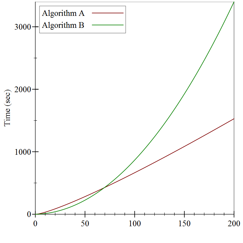
It turns out that while Algorithm B started off faster than Algorithm A, it wasn’t by much, and it didn’t last very long: even for reasonably small inputs (only 60 items or so), Algorithm A winds up being substantially faster.
We have to be quite careful when talking about performance: a program’s behavior on small inputs typically is not indicative of how it will behave on larger inputs. Instead, we want to categorize the behavior as a function of the input size. As soon as we start talking about “categories”, though, we have to decide just how fine-grained we want them to be.
For example, the graphs above supposedly measured the running time of these two algorithms in seconds. But they don’t specify which machine ran the algorithms: if we bought a machine that was twice as fast, the precise numbers in the graphs would change:
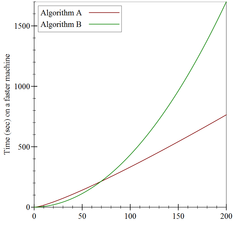
But the shapes of the graphs are identical!
Surely our comparison of algorithms cannot depend on precisely which machine we use, or else we’d have to redo our comparisons every time new hardware came out. Instead, we ought to consider something more abstract than elapsed time, something that is intrinsic to the functioning of the algorithm. We should count how many “operations” it performs: that way, regardless of how quickly a given machine can execute an “operation”, we have a stable baseline for comparisons.
27.2.2 ...and space
The argument above shows that measuring time is subtle, and we should measure operations instead. An equivalent argument shows that measuring memory usage is equally tricky: objects on a 16-bit controller (like old handheld gaming devices) take up half as much memory as objects on a 32-bit processor, which take up half as much memory again as on 64-bit machines... Instead of measuring exact memory usage, we should count how many objects are created.
27.2.3 It was the best of times, it was the worst of times...
In fact, even measuring operations (or allocations) is tricky. Suppose we were asked, in real life, to sort a deck of cards numbered 1 through 100. How long would that take? If the deck was already sorted, it wouldn’t take much time at all, since we’d just have to confirm that it was in the correct order. On the other hand, if it was fully scrambled, it might take a while longer.
Likewise, when we analyze algorithms for their running times, we have to be careful to consider their behaviors on the best-possible inputs for them, and on the worst-possible inputs, and (if we can) also on “average” inputs. Often, determining what an “average” input looks like is quite hard, so we often settle for just determining best and worst-case behaviors.