Computer Graphics (CS 4300) 2010S: Lecture 20
Today
- lights: ambient, point, directional, and spot
- simplified local light-surface-eye geometry
- diffuse (Lambertian) shading
- specular (Blinn-Phong) shading
- ambient and emissive shading
- Gouraud interpolation, “flat” vs “smooth”, and per-vertex vs per-fragment shading
Lights
- so far, when we rasterize any primitive larger than a point (i.e. a line segment or a triangle), we know how to interpolate the color of any fragment inside that primitive given the colors at the vertices
- we have treated the vertex colors simply as inputs to the process, just like the vertex positions (i.e. in your homework assignments, you read both the positions and the colors from an input file)
- for a triangle, you use barycentric interpolation to determine fragment color; for a line segment you’d just use linear interpolation
- the results can produce a reasonable image, but for many 3D shapes it is hard to see the surface geometry because so far we have not accounted for any of the actual interactions of light sources
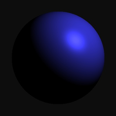
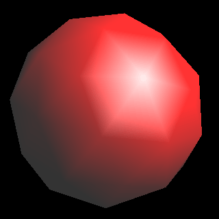
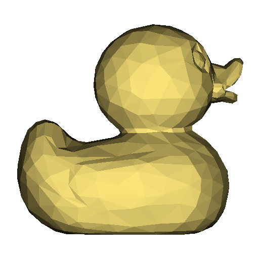
- for example, as you have seen, many models actually specify the same (or nearly the same) color at many (or all) vertices; in this common case, interpolating the vertex colors just ends up copying the same color to every fragment, as shown in the left image below
- if we do the same thing but first modulate the vertex colors according to a model of the interaction of the surface with some light source, we can get an image like the one on the right below, which is much better (this particular rendering is an instance of flat shading, which as we will discuss below, is just one form of computing light interaction)

- in all of what follows, we will make many approximations of reality: the way light sources actually behave, the way light actually interacts with surfaces, the way it travels through the air or other translucent media, and the way it interacts with your eye, are all much more complex in reality
- since shading computations typically need to be done very quickly, it is common (at least in real-time graphics) to make many approximations
- these are effectively heuristics that people have come up with over the years
- the results can look reasonable, but are usually not perfect
- nevertheless, they can be “good enough”, and much better than doing nothing at all
- the first thing we need to simulate the effect of light interacting with a model, also simply called shading, is to define some light sources
- four types of light source models are common in real-time graphics
- a point light is like a totally symmetric light bulb situated at some point in space
- it radiates light from that point equally in all directions
- a point light can thus be defined by specifying a 3D point
 and a light intensity
- while it is entirely reasonable to consider
 to be a scalar, in which case we typically consider the light source to be colorless (or, simply, white), it is actually most common in graphics implementations to let
  be a vector
  , which specifies the intensity of the light specifically in red, green, and blue
 - this is like having a colored light source, or, equivalently, one red, one green, and one blue light bulb that are each “turned on” to an extent proportional to the corresponding component of

- while the rays emanating from a point light go off in all directions, a directional light is like an infinite glowing plane: it casts all its rays in parallel along a specific direction
- thus a directional light can be defined by its direction, typically a unit vector
 , and again by an intensity which may either be a scalar
  or a vector (for a colored light)
- while the description of directional light may so far seem very unnatural, in fact it is a very good approximation of a common real-world situation: illumination by a very distant point source, such as the Sun
- even though the Sun technically radiates light in all directions (it is not really a point, as we know, but more like a glowing sphere), because it is so far away, all the rays that end up near some specific location on the surface of Earth must all be very nearly parallel
- a third kind of light combines aspects of both point and directional lights: a spot light simulates the kind of light that could be given off by a typical desk lamp
- a spot light has both a location
 and a direction
- it further has an angle
 , which typically defines a symmetric cone of rays emanating from
  around the center direction
- like all lights, it also has either a scalar
 or vector (colored)
  intensity
 - sometimes spotlights are also defined with an attenuation factor
 so that the light is brightest along
  and dims as the edges of the
  cone are approached
- the final common type of light source is an ambient light, which effectively is “everywhere”
- ambient light has neither a defined position nor direction, just an intensity
 or
or 
- this is an approximation of a common effect in the real world: light reflects off objects so that the total incident light at any given point on a surface effectively includes a random component of rays from various directions
- as we will see, it is not common in real-time graphics to explicitly model reflections, but we can recover the effect of this indirect lighting by explicitly adding some ambient light
- generally, zero or more lights can be defined in any 3D scene in practice, some libraries, such as OpenGL, can enforce limits on the total number of lights
- the more lights, the more calculations that need to be performed for shading
- OpenGL is often an interface to specialized graphics hardware, and that hardware classically only included capacity for a limited number of light sources
- simple applications typically define only a few lights, e.g. ambient and one directional light
- more complex applications might also model specific light sources in the scene, such as streetlights or indoor lamps
Light-Surface-Eye Geometry
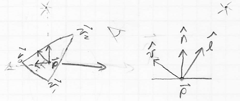
- now that we have both some geometry and some lights, we can set up the math to model their interaction
- we will do this at the level of one primitive
- specifically, we will consider a triangle, because it is the main primitive used to model object surfaces that reflect light
- it is sufficient to draw a 2-D picture that shows the triangle edge-on

- at any given 3D point
 on the triangle, three unit vectors are fundamental
- the outward pointing surface normal

- we know that
 can be computed directly from the vertices of the triangle
 - e.g. if the vertices are
 , then we can define
  and then
  (this is what you have done in homeworks so far)
 - this is true if the triangle is truly flat
- in fact there are other ways to come up with
 that simulate triangles with curved surfaces; we will discuss this more later
- the vector
 from that point towards the viewer
- for perspective projection, this is literally the vector from
 to the origin of camera frame (as we have defined it)
 - for parallel projection, this is just the
 axis of the camera frame (as we have defined it); with no dependence on
- the vector
 from that point towards a light source
- this assumes either a point, directional, or spot light; we will discuss ambient light later
- if there are multiple lights, we deal with them one at a time, and then simply add the resulting colors at the end
- for a point or spot light at location
 , this is just the unit vector
- for a directional light with direction
 ,
, 
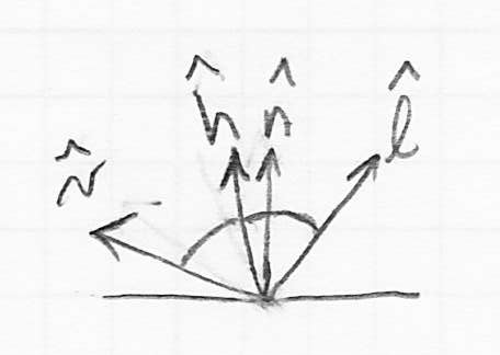
- a fourth unit vector is often derived from
 and
and  :
:  is the vector halfway between
  and
and 

- this can be calculated as the average of
 and
and  :
:  , and
, and 
- note that since we are normalizing the vector length anyway, we don’t really need to divide by 2; we can just directly calculate

Diffuse (Lambertian) Shading
- in the 18th century a scientist named Lambert noticed that the apparent illumination of a surface is reasonably approximated by the cosine of the angle between the surface normal of the light source
- because we have defined all our vectors with unit length, we can easily calculate this cosine as the dot product

- the result is non-negative as long as the surface is not “facing away” from the light source
- as long as that is true we can calculate the diffuse shaded color
 of the surface at point
  as
as  (otherwise there is no diffuse contribution for this light at
  )
)- where
 is the diffuse color of the surface, which could be e.g. the original unlit color that would be returned by barycentric interpolation of the input vertex colors
 - the operator
 is an element-by-element multiplication of two vectors, i.e.
 is the color of the light source as defined above
 is the unit vector from the surface point to the light source
 is the unit surface normal
Specular (Blinn-Phong) Shading
- diffuse shading is much better than no shading, but always yields matte surfaces that can look very “chalky”
- in reality, many surfaces also act at least a little bit like mirrors
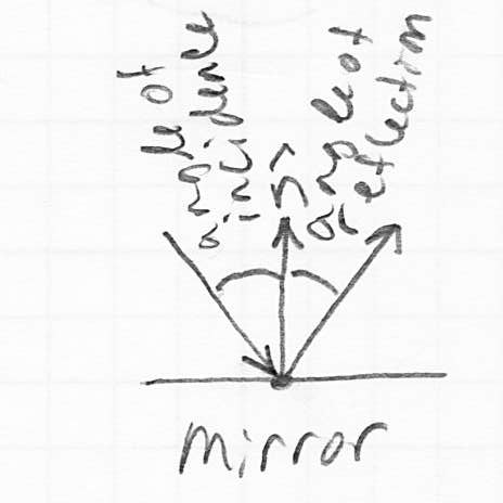
- how does a mirror act?
- a perfect mirror reflects each incoming light ray along an output direction that is symmetric with respect to the surface normal
- mirror law: “the angle of incidence equals the angle of reflection”

- we can simulate this effect by adding a term to the above equation:

- here
 is the vector halfway between
  and
and  (the unit vector towards the viewer)
 - taking the dot product of
 and
and  is a heuristic that approximates how close to the mirror output direction the viewer currently is
  is a constant called the Phong exponent (typically around 20 or higher), that controls the tightness of the resulting specular highlight
 is the specular color of the surface, which can be the same as
  , or could be different for some added flexibility
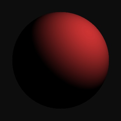
- the image at left below has only diffuse shading, the image at right has both diffuse and specular:


Ambient and Emissive Shading
- finally, we may add both ambient and emissive terms to our shading equation:

 is the ambient color of the surface
 is the emissive color, which can model surfaces that glow (although note that these are not true light sources, as they do not illuminate anything else in the scene)
- note that after adding up all these different terms, it is entirely possible to end up with components of
 that are greater than one; in practice we simply clamp the resulting color components to the range
- we may also have multiple light sources; we just add up all their individual effects
- in practice, it is common to assume that point, directional, and spot lights only contribute to the diffuse and specular terms in the shading equation, and that a separate ambient light (typically there is at most one ambient light) contributes only to the ambient term
- we now return to the idea of how to calculate the surface normal
 at a given point on a triangle
 - it may seem that we have no choice but to take the cross product of two sides of the triangle
- if the triangle is truly flat, then the surface normal is the same everywhere, and must be equivalent to such a cross product (when the result is normalized)
- however, as you know, it is common to use a mesh of triangles to approximate a surface that is not actually flat
- if the individual triangles are small enough, then the resulting shading does begin to approximate the appearance of the actual curved surface
- even though each triangle will individually appear flat (in fact, this whole approach is called flat shading), we can use a lot of very small triangles to minimize the artifact of seeing the individual facets
- technically the
 and
and  vectors, as well as the barycentric interpolated base color
  , can still vary among the fragments of the triangle
 - but in some common implementations, such as OpenGL, the term “flat shading” refers to an even simpler model, where the shaded color is calculated for just one (typically the first) vertex of the triangle, and then copied exactly across the entire triangle
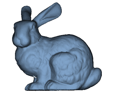
- below we see the “bunny” model rendered with 500, 1000, 10000, and ~70000 facets


- it turns out that if we are willing to make our computation of the normal vector a little more complicated, we can do much better than flat shading
- the main idea is to no longer imply the surface normal from the triangle itself, but rather to read in normal vectors as an additional property of every vertex, just like we already read in the vertex colors
- this allows the modeling application (which generates input files like the duck and bunny that we’ve been using) to calculate and specify the actual surface normal at the vertices

- note that for a curved surface, this can in general be different from the surface normal of any of the adjacent triangles

- what if the input file does not include vertex normals?
- recall the input files in your homework define only the position and color of each vertex
- one approach is
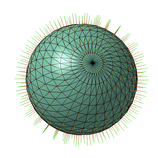
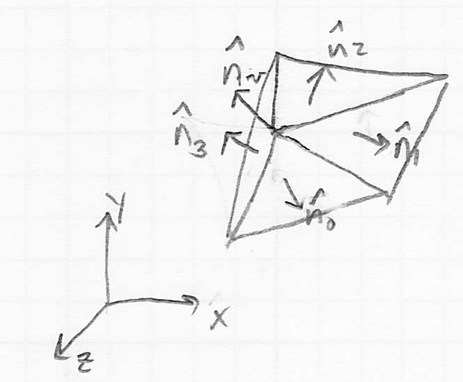
- compute the flat surface normals of all triangles adjacent to a given vertex
- take the average of all those, normalize it, and set that as the normal at the vertex
- this gives us all the information we need to calculate accurate curved-surface shading at each vertex
- but what about the fragments in the interior of a triangle?
- one thing we can do is just do the full shading calculation at the vertices and then use barycentric interpolation as a heuristic to approximate the shaded colors for a curved surface at the interior fragments
- this is called Gouraud interpolation
- it works ok in practice, especially if the triangle mesh is not too coarse, but can produce visual artifacts
- prior to programmable fragment shaders, this was the main approach to “smooth” shading in APIs like OpenGL
- now it is possible to also implement per-fragment shading, which interpolates the normal vector (again using barycentric interpolation) and then does the full shading calculation per-fragment
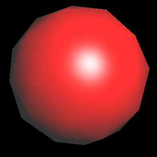
- on the left below are coarsely tessellated spheres showing rendering artifacts using Gouraud interpolation; on the right the corresponding images are shown with per-fragment shading (images from opengl.org)


Limitations of the Standard Real-Time Light Model
- the above issues with Gouraud interpolation are one major issue with this overall approach to lighting
- some other big ones:
- we have not modeled shadows
- we have not modeled light that reflects off one object and hits another
- we have not modeled refraction of light through translucent materials
Next Time


 and a light intensity
 to be a scalar, in which case we typically consider the light source to be colorless (or, simply, white), it is actually most common in graphics implementations to let
  be a vector
  , which specifies the intensity of the light specifically in red, green, and blue
 , and again by an intensity which may either be a scalar
  or a vector (for a colored light)
 and a direction
 , which typically defines a symmetric cone of rays emanating from
  around the center direction
 or vector (colored)
  intensity
 so that the light is brightest along
  and dims as the edges of the
  cone are approached
 or
or 
