Computer Graphics (CS 4300) 2010S: Lecture 13

Today

• procedural and approximating curves
• cubic Bézier curves and splines
• de Casteljau algorithm

Procedural and Approximating Curves

• so far we have studied two ways to define curves—parametric and implicit forms—as well as the idea of defining a curve or spline by a set of control points that must be interpolated (i.e. that the curve must “go through”)
• today we generalize both of these a little bit
  • we will introduce a third way to define a curve, simply as a computational procedure that produces points on the curve (yes, this is a generalization of the parametric approach)
  • we will study approximating curves that are specified by a set of control points, but which do not necessarily interpolate all of them
• why?
  • we can still interpolate some of the points, and we can use the remaining ones to control the shape of the curve between those
  • we can implement very efficient algorithms for operations on these kinds of curves, including drawing them, splitting them into smaller parts, etc.
• in fact, we will study both in the context of a single very important curve formulation: Bézier curves

Cubic Bézier Curves and Splines

• one way to start thinking about Bézier curves is to consider them a generalization of Hermite cubics
• Bézier curves can in fact be defined for any degree, though it is most common in graphics to deal with the cubic case
  • as we have already seen, a single cubic piece is very useful: since it can bend twice, we can independently specify both the start and end points and also the start and end tangents
  • we can then string together cubic pieces into a spline for more complex curves
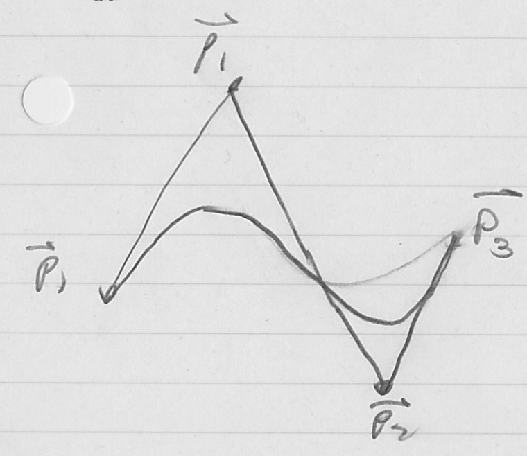
• the idea of a cubic Bézier curve starts with a four point control polygon
  • examples
    
    
  • (this is one of those cases where we use the word “polygon” to refer to a piecewise linear curve that is not actually closed; i.e. we don’t normally think of the segment as part of the control polygon for a cubic Bézier curve; the control polygon thus is just an open chain of the three segments , , )
  • the curve starts at and ends at
  • the tangent at the start of the curve is , i.e., it is a scaling of a vector along the first side of the control polygon by the degree of the curve
  • the tangent at the end of the curve is , i.e. it is a scaling of a vector along the third (last) side of the control polygon by the degree of the curve
  • so the curve is totally defined by its control polygon
  • in fact, in a way that we will make precise shortly, the curve is essentially a “smoothing” of the control polygon
• we will focus on the cubic case, but generalizations to higher degree are similar: the control polygon always has points, and the first derivatives of the curve are defined at both the start and the end points by the nearest points on the control polygon
• as before, we can set up a system of linear equations to solve for the coefficients of a cubic vector polynomial
  • let ,
  • use the definition , so
  • then the start and end location constraints give
  • 
  • 
  • and the start and end tangent constraints give
  • 
  • 
  • as for the Hermite formulation, two of the coefficients are determined directly
  • and
  • 
  • but we have to solve a linear system to find expressions for (we can re-use the answer from the Hermite form, but then simplify)
  • 
  • 
  • putting these all together, we have
  • in the analysis of Bézier (and related) curves, it is common to re-group the terms like this:
    • this is called the Bernstein form
    • it generalizes with a simple pattern to arbitrarily high degree
    • it can be more efficient and more accurate to calculate
    • it also is more amenable to some kinds of analysis
    • you should be aware of it, but we won’t study it further in this course
• properties of Bézier curves
  • besides what we already know (that the curve interpolates the first and last points of its control polygon, and that its tangents are defined by the first and last segments of the control polygon), Bézier curves have some very useful properties
  • any Bézier curve is always bounded by the convex hull of its control points
    • this is very useful for example to quickly check if two Bézier curves do not intersect
  • any line intersects the curve no more times than it intersects the control polygon; this is called the variation diminishing property, and relates to the idea that the curve is a smoothing of the control polygon
  • Bézier curves are affine invariant: affine transformations (rotation, translation, reflection, scale, shear) applied to the control points result in a Bézier curve with the corresponding transformation
  • Bézier curves are easily subdivided (split into two pieces that are themselves Bézier curves of the same degree)—we will see an algorithm to do this later
  • Bézier curves are reversible: the vertices of the control polygon taken in reverse order yield the same Bézier curve but with reversed parametrization
• cubic Bézier splines with cubic Bézier pieces are simple to form: just start with a control polygon with vertices
  • then the -th piece, for , is a cubic Bézier curve defined by the control points
  • the spline has (position) continuity by construction
  • (geometric tangent) continuity can be maintained at any (or all) knots as desired by ensuring that the adjacent control polygon segments are collinear
  • (parametric tangent) continuity can similarly be maintained by ensuring that the control polygon segments adjacent to a knot are both collinear and the same length
• two other common kinds of splines, B-Splines and Non-Uniform Rational B-Splines (NURBS) are related to, but not the same as, Bézier splines
  • they are a bit more complex, and we will not study them in this course
  • they offer both more control (for example, to easily maintain or higher continuity) and more capability (for example, NURBS can exactly represent a circle, whereas Bézier and B-splines can only approximate circles)

de Casteljau Algorithm

• we now have a parametric polynomial formula for a Bézier curve, so given a parameter value we can compute the coordinates of the corresponding point on the curve
• one way to draw the curve is to repeatedly compute such points for a whole set of parameter values, and then to connect the resulting sample points on the curve with line segments
• but how many sample points are necessary and sufficient, and how should they be distributed?
• we will give one method to resolve this question, but first we must introduce an important algorithm for Bézier curves
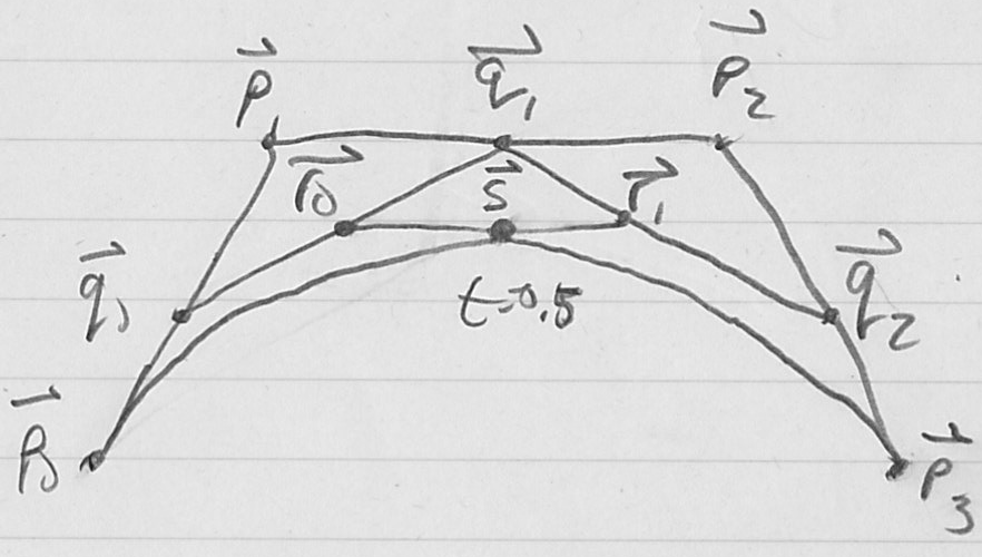
• while we can use the parametric formula to find the coordinates of a point on the curve corresponding to a given parameter value, there is an alternative procedural form for finding the point, called the de Casteljau algorithm
• let the input be the control polygon and the desired parameter value at which to compute the output point
  1. compute
     • 
     • 
     • 
  2. compute
     • 
     • 
  3. compute
     • 
• graphically, this looks like we are twice “cutting off the corners” of first the original control polygon
  
  • this is an example of a subdivision scheme; there are other related methods in graphics, mainly for creating smooth curves and surfaces
• the de Casteljau algorithm generalizes directly to Bézier curves of any degree
  • the number of points “in play” starts with the size of the control polygon, which is always , and is reduced at each stage by 1
• an extremely useful feature of the de Casteljau algorithm is that the intermediate points it computes actually form two smaller Bézier control polygons which correspond to Bézier curves from to and from to
  • the control polygon for the first sub-curve is
  • the control polygon for the second sub-curve is
• recalling the convex hull property (that a Bézier curve is always bounded by the convex hull of its control polygon), this actually suggests an answer to the question of how to select an ideal set of sample points when drawing a Bézier curve as a chain of line segments
  1. first, check if the original Bézier curve is already “close enough” to a line segment by checking if the vertices of its control polygon are already “near enough” (i.e. within one pixel) of collinear
  2. if so, just draw a line segment from to . Done.
  3. otherwise, split the original Bézier curve into two pieces at using the de Casteljau algorithm, and recur (i.e. start back at step 1) with each piece!

Next Time

• reading on website
• pose interpolation in 2D
• keyframe animation
• navigating in 2D

this page subject to change  |  last updated Mon Apr 19 13:06:46 EDT 2010  |  course homepage