Computer Graphics (CS 4300) 2010S: Lecture 12
Today
- HW3 due next Thurs Feb 25 at 12pm
- midterm moved to Mon March 8 (first day back after spring break)
- piecewise parametric curves in 2D
- polynomial curves in 2D
- interpolating curves in 2D
Piecewise Parametric Curves
- last time, we defined a parametric curve to be a pair
 where
where is a specific parameter interval
 is a vector-valued continuous function
- but we only gave a few specific parametric curves
- these included line segments and circles (among others)
- actually, we only defined “full” circles, but it’s straightforward to limit the parameter space to get a part of a circle, i.e., a circular arc
- what if we want a curve where e.g. some parts are line segments, and some parts are circular arcs?
- in code, we could just represent this as a list datastructure where the list elements are either line segments or circular arcs, provided that we also maintain the invariant that the endpoint of one element must equal the starting point of the next
- in math, we define a piecewise parametric curve
- for simplicity, assume we only have two “pieces”
- let
 be the first piece, with
- let
 be the second piece, with
- also, assume that
 , which will ensure
  continuity of the final result
 - then
 and
and  constitute a curve where the second piece is “pasted” onto the end of the first
 - the location
 in
in  is called a knot
 - the method extends directly to
 pieces
  defined over any closed domains
  with any final closed domain
  and knots
Polynomial Curves
- as you likely know, a polynomial is an expression of the form

- the
 are constant coefficients
  is the degree of the polynomial
- in particular
- degree 1 polynomials are linear
- degree 2 polynomials are quadratic
- degree 3 polynomials are cubic
- if we use 2D vectors as coefficients, then we can easily define a parametric curve with a polynomial vector function:

- simple example: the line segment
- intuitively, a line segment should be representable as a linear polynomial:

- in this simple case, the geometric meaning of
 is not too hard to figure out
 is the starting point of the segment
 is the
  vector we have discussed: a vector from the start to the end of the segment
- for higher-degree curves, the meaning of the
 coefficients is less obvious, and we will study ways to calculate their values based on more geometrically meaningful attributes of the curve
- polynomial curves are mainly useful because for
 they can bend!
- linear polynomial curves have no bends
- quadratic polynomial curves have at most one bend
- cubic polynomial curves have at most two bends
- can any curve be exactly represented as such a parametric polynomial?
- no! a circle is one example…
- however, especially when we form piecewise curves with polynomial parts, we can at least approximate a large number of useful curves
- in fact, in graphics it is common to use only parts that are either linear, quadratic, or cubic
- and since quadratic and linear polynomials are degenerate cubics, we can focus primarily on cubics
- a cubic parametric polynomial curve (or just a cubic curve) can be written

- any cubic curve is specified by selecting values for the constants

- but what relation do these constants have to the shape of the curve?
- in fact, the connection is generally not obvious
- what kinds of attributes might we want to actually control?
- one way to look at the problem is to recall the local curve properties we defined last time
- we might want the curve to go through, or interpolate a particular point
 at specific parameter value
  :
: 
- we might want the curve to have a certain local tangent vector
 at a specific parameter value
  :
: 
- we might want the curve to have a certain local normal vector (and hence a specific curvature)
 at a specific parameter value
  :
: 
- observe we have four “knobs” that we can turn:

- this means that if we specify four independent constraints on the curve, i.e. if we specify the desired position, tangent, or normal of the curve at four places, then all the
 will be determined
 - one obvious case for a cubic curve would be to specify four points
 that must be interpolated at specific parameter values
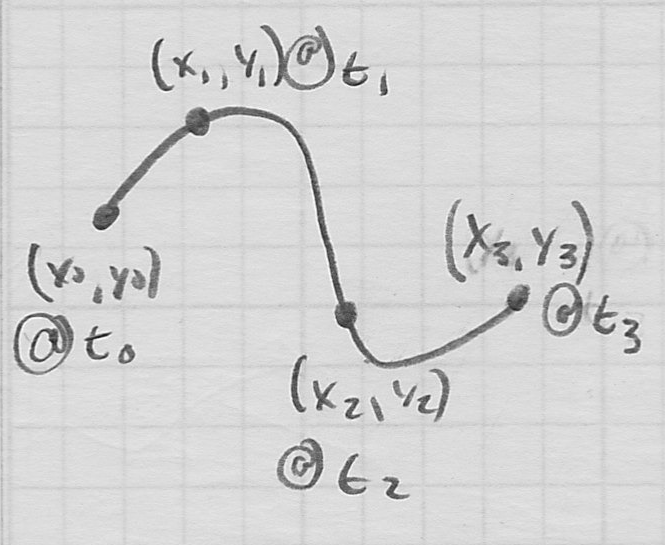
- another interesting way to specify a cubic is to give desired start and end points
 and also desired start and end tangents
- this is called the Hermite form
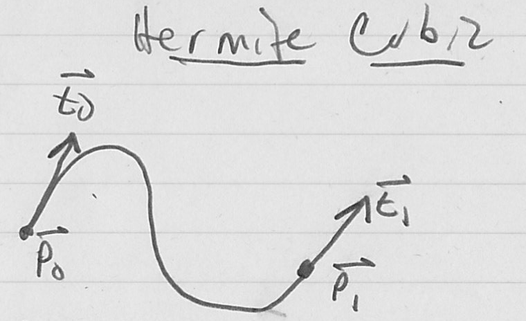
- assume the parameter domain is

- recall the basic definition of a general cubic curve:

- now apply the start and end location constraints


- and the start and end tangent constraints, using


- so
 have already been determined:
  ,
, 
- to compute
 we need to solve the remaining system of two linear equations in two unknowns

Interpolating Curves
- though there are different geometric attributes we may want to control at different times (e.g. we just saw control of both position and tangent), a common case is to specify at least some points that we would like a curve to interpolate
- next time we will also study the related case of approximating curves that merely pass “near” some specified points
- interpolating polynomials
- an
 -degree vector polynomial has
  coefficients
- remember, these are “knobs” we can turn to shape the curve
- if we specify
 independent constraints, we will totally define the curve
 - so we may specify
 points
  to interpolate at corresponding parameter values
- e.g. for a cubic curve,
 and we have the following system of four constraint equations:


- be careful! In this setting, the
 are the variables we are solving for, and the
  and
and  are constants
 - we thus have a linear system of 4 equations in 4 unknowns (or, in general,
 equations in
  unknowns)
 - if
 then
then  so
so 
- there is guaranteed to be a unique solution as long as all
 are different
 - it is theoretically possible to interpolate any number of points by using a single polynomial of sufficiently high degree
- but this is not commonly done, partly because it’s computationally expensive, but also because it is hard to manage from a user interface perspective
- one major issue is that the shape of the resulting curve is non-local with respect to changes in a single point
- i.e. moving just one of the interpolating points
 may change the shape of the entire curve (it will still go through all the other points, but the “in-between” parts can, and generally will, change)
- similarly, to evaluate the curve, i.e. to find the coordinates of a point at a given parameter value along the curve, requires a computation that in general will involve all the points

- solution: use a piecewise curve
- Hermite splines
- back in the dark ages, before computers, when a draftsman wanted to draw a curve other than a circle or ellipse, one tool he or she could use was a spline: a long piece of bendable rubber that would hold its shape so that it could be traced
- this terminology has carried over to the modern algorithmic implementations of the same kind of functionality
- there are a variety of ways to implement splines. We will cover several.
- in general, splines are defined as piecewise curves
- some of the more simple common approaches are actually piecewise polynomial
- one of the simplest is the Hermite spline
- recall that the Hermite form for a cubic curve allows the starting and ending locations and tangents to all be specified independently
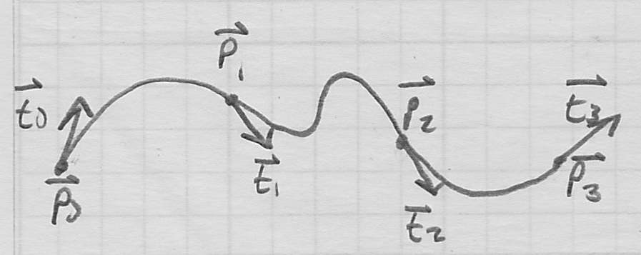
- given a list
 of points and a second list
  of tangent vectors
 - construct a piecewise curve by defining
 Hermite cubic pieces
 - the
 th piece starts at
  and ends at
  , and has starting tangent
  and ending tangent

- the result interpolates all the
 and is both
  and
and  continuous by construction
 - note that modifications to the
 and
and  only affect the two adjacent curve pieces, i.e., modifications to the control parameters are local
 - similarly, to evaluate the spline, i.e. to find the coordinates of a point at a given parameter value, involves only a computation on the
 and
and  for one of the curve pieces
 - one issue to be solved when implementing is how to present a reasonable UI for specifying and modifying the

- cardinal cubic and Catmull-Rom splines
- in many cases we would like to specify a set of points to interpolate, and we would also like
 continuity (
 continuity is implied by the fact that we’re constructing a single spline curve), but we don’t care so much about the exact tangent vectors
 - so we would like an algorithm that “figures out” reasonable tangent vectors to assemble a
 piecewise cubic through a given set of points
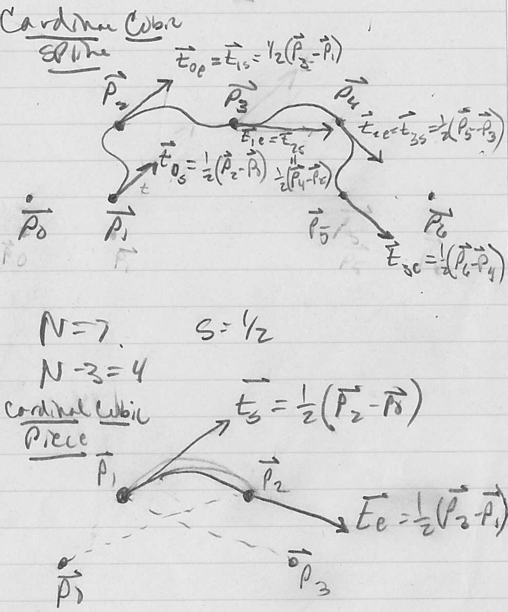
 - one common approach is the cardinal cubic formulation
- given a set of points
 ,
, 
- and a single additional tension parameter

- the cardinal cubic formulation computes the coefficients
 for a set of
  cubic pieces (i.e.
  ) that
 - interpolate
 through
  in order (i.e. all but the first and last of the given points)
 - maintain
 (position) and
  (tangent) continuity
 - has a “sharpness” of turns at the interpolation points controlled by

- example with


- we will now derive the equations to compute
 for a given piece
  , i.e.
  , with
- we know that the curve must interpolate
 and
and  , so we have the first two constraints:

- now we will construct tangent constraints by using the vector from
 to
to  as
as  and the vector from
  to
to  as
as  . In both cases, we scale the tangent by the tension parameter
  :
: 

- for
 ,
,  , ensuring tangent continuity
 - we can finally be quantitative about the meaning of

- for
 the tangents have zero length, and this enables the “sharpest” turns: each piece of the spline is actually just a line segment (in fact, in this case,
  continuity still holds, but only on the technicality that the tangents are actually zero at the interpolation points)
 - for increasing
 the tangents have increasing length, and correspond to “smoother” turns
 - the case
 is a common choice, and is called a Catmull-Rom spline
- again,
 are directly computed, but we need to solve a
  linear system for
  :
: 

- cardinal cubic splines thus have many of the same advantages as Hermite splines (
 and
and  continuity, local control, local evaluation) but do not require the user to specify details of tangent vectors
 - Catmull-Rom splines don’t even require setting a tension (by definition, they are just cardinal cubics with tension 0.5)
- one drawback is that cardinal cubics do not interpolate the very first or the very last of the given points
- this is easily resolved in practice by inserting two “dummy” points, one before and one after the points given by a user
- Catmull-Rom (and some similar) splines are commonly used in particular to interpolate animation parameters, as we will see later in the course
Next Time
- reading on website
- approximating curves in 2D
- Bézier curves and splines in 2D
 is a specific parameter interval
 is a vector-valued continuous function
 be the first piece, with
 be the second piece, with
 , which will ensure
  continuity of the final result
 and
and  constitute a curve where the second piece is “pasted” onto the end of the first
 in
in  is called a knot
 pieces
  defined over any closed domains
  with any final closed domain
  and knots


 then
then  so
so 
